Generalizing Attention in NLP and Understanding Self-Attention
Generalizing the idea of attention in NLP and understanding various methods of calculating attention used in the literature so far. Also, understand and implement multiheaded self-attention using PyTorch.


- Introduction
- Introduction to Attention in NLP
- Generalizing Attention
- Multiheaded Self Attention
- References
Introduction
Attention is one of the most important and ubiquitous concepts in NLP and deep learning. There are many blog posts out there explaining different flavors of attention. This blog post however, introduces attention as a general concept in NLP and then goes onto explain some of the most important methods of calculating attention vectors. Each sub-topic or concept is concretely supported by real-world intuitions. Lastly, this post explains the idea of multiheaded self-attention in a unique by using the idea of linear projections and concludes by showing stepwise how to translate all the intuitions to code.
This blog post is a small excerpt from my work on paper-annotations for the task of question answering. This repo contains a collection of important question-answering papers, implemented from scratch in pytorch with detailed explanation of various concepts/components introduced in the respective papers.
Introduction to Attention in NLP
Attention as a concept in NLP was introduced in 2015 by Bahdanau et al. to improve neural machine translation systems. Before this paper, NMT systems were largely based on seq2seq architectures which had an encoder to encode a representation of the source language and a decoder which to decode this representation into the target language. Such models were trained on large quantities of parallel text data of two languages. One major drawback of this architecture was that it didn't work well for longer documents/sequences. This is because the entire information in the source sentence was being crammed into a single vector. If this vector fails to capture the important information from the source language, the system is going to perform poorly.
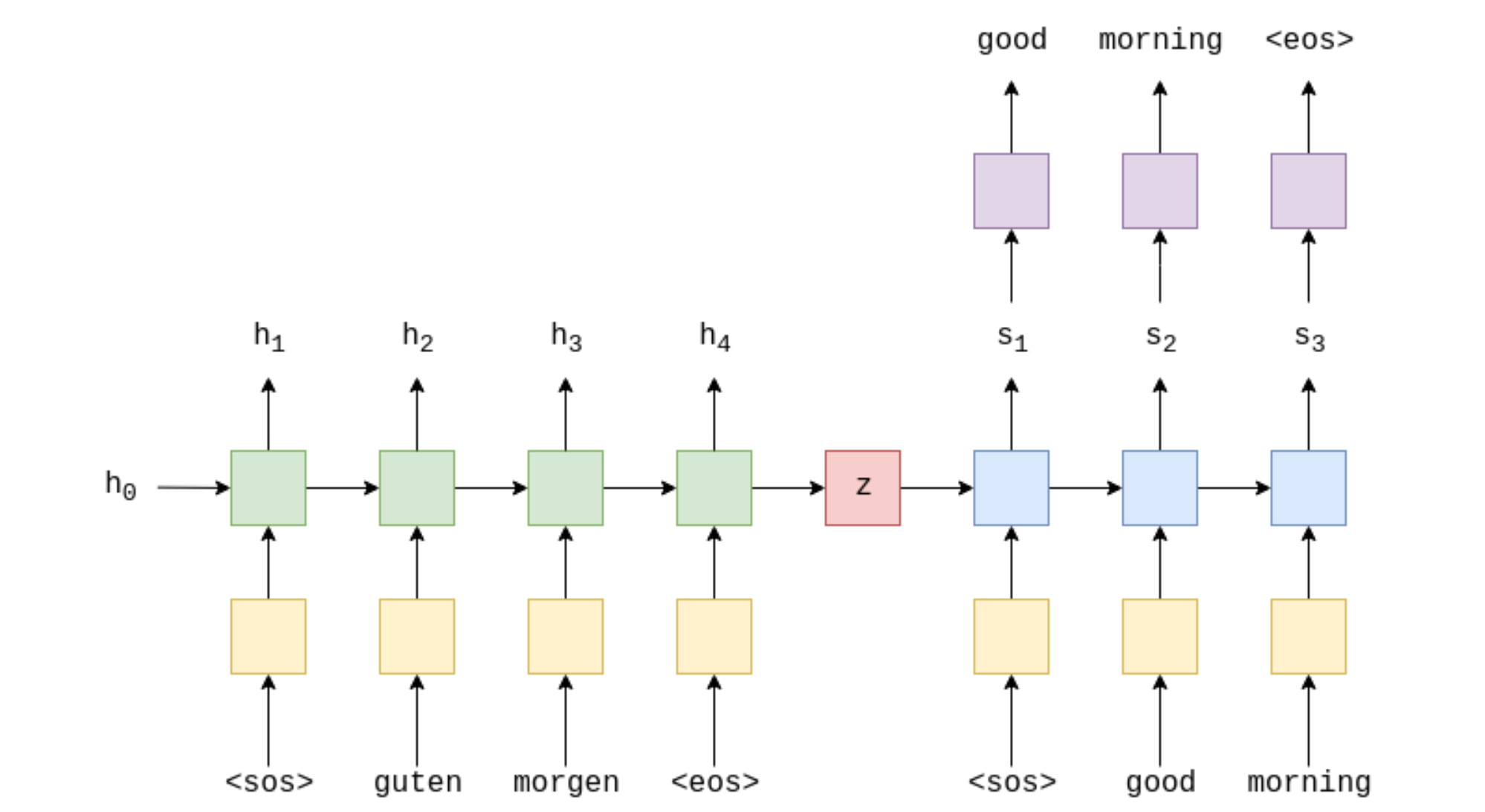
When we claim that these neural nets mimic the human brain, this is certainly not how the human brain works. While learning about some topic, we do not simply read 2-3 pages of content and expect our brain to remember all the details in the first go. We usually revisit various concepts, recollect and refer to the material back and forth before mastering it. The attention mechanism in NMT was designed to do this. While decoding at any particular time step, encoder hidden states from all the time-steps are made available to the decoder. The decoder then can look back at the encoder hidden states or the source language and make a more informed prediction at a particular time-step. This alieviates the problem of all the information from source language being crammed into a single vector.
To illustrate this with equations, consider that the hidden states of the encoder RNN are represented by $H$ = {$h_{1}, h_{2}, h_{3},...,h_{t}$}. While decoding the token at position $t$, the input to the decoder unit is hidden state from previous unit $s_{t-1}$ and an attention vector which is a selective summary of the encoder hidden states and helps the decoder to pay more attention to a particular encoder state.
The similarity between the encoder hidden states $H$ and the decoder hidden state so far $s_{t-1}$ is computed by,
$$ \alpha = tanh (W [H ; s_{t-1}]) $$
$\alpha$ is then passed through a softmax layer to obtain attention distribution such that $\sum_{t} \alpha_{t}$ = 1. The final step is calculating the attention vector by taking a weighted sum of the encoder hidden states, $$ \sum_{t} \alpha_{t} h_{t} $$
The following diagram illustrates this process.

Since then, many different forms of attention have been proposed and used in the literature. Attention is not limited to NMT systems and has evolved into a more general concept in NLP. At the heart of it attention is about summarizing a particular entity/representation by attending to the important parts of this representation. A more general definition of attention is as follows:
Given a set of vectors
values, and a single vectorquery, attention is a method to calculate a weighted sum of the values, where the query determines which values to focus on.
It is a way to obtain a fixed size representation of an arbitrary set of representations (values), dependent on some other representation (query).
In our earlier NMT example, the encoder hidden states {$h_{1}, h_{2}, h_{3},...,h_{t}$} are the values and the decoder hidden state $s_{t-1}$ is the query.
Generalizing Attention
In general there are 3 steps when calculating the attention. Consider that values are represented by {$h_{1}, h_{2}, h_{3},..h_{n}$} and query is $s$. Then attention always involves,
- Calculating the energy $e$ or attention scores between these 2 vectors, $e$ $ \epsilon$ $ R^{N} $
- Taking softmax to get an attention distribution $\alpha$, $\alpha$ $\epsilon$ $R^{N}$
$$ \sum_{t}^{N} \alpha_{t} = 1 $$
- Taking the weighted sum of the
valuesby using $\alpha$ $$ a = \sum_{t}^{N}\alpha_{t}h_{t} $$
Now there are different ways to calculate the energy between query and values.
Basic Dot Product Attention
$$ e_{t} = s^{T}h_{t}$$Additive Attention
$$ e_{t} = v^{T} tanh (W [h_{t};s])$$
This is nothing but the Bahdanau attention attention first proposed for NMT systems.
Bilinear Attention
$$ e_{t} = s^{T} W h_{t}$$ where $W$ is a trainable weight vector. This has been used extensively in Question Answering systems like the Stanford Attentive Reader and DrQA
Scaled Dot Product Attention
$$ e_{t} = s^{T}h_{t}/\sqrt n$$ where $n$ is the model size. A modified version of this proposed in the Transformers paper by Vaswani et al. is now employed in almost every NLP system. The following section explains this attention in more detail.
Multiheaded Self Attention
Idea of Linear Projections
Consider a system of an online book store like kindle, which lets you rent, buy and read books on its platform. Such platforms usually have a recommendation system (recsys) in place that enables them to understand their users' taste and preferences over time. This helps them in making personalized recommendations to users and in turn improve their revenue. For simplicity, let's assume that there are 10,000 books available on the platform and the system maintain a simple binary vector of size 10,000 for each user. If a user has read a particular book, the position in the vector corresponding to the book's id is 1 and 0 otherwise. A books-read vector for a user looks like, $$ [1,0,0,1,1,0,0,0,0,1,1,...,1] $$
Now assume a projection matrix of dimension 10,000 X 100. When we multiply any user's books vector, we get a new low dimensional vector of size 100. This vector is totally different from the previous one and now represents the user's taste or preferences in books. It basically represents a user-profile for the recommendation system. Calculating this user-taster vector for different users enables the application to find users with similar taste and recommend books that they might like simply based on what the other "similar" user has read.
The weights or values of this projection matrix can be thought as representing certain features or properties that a book might possess. It might capture various genres like science, philsophy, fantasy novels, etc.
The question that still remains however, is how do we get such a projection matrix in the first place that can transform a represenation from one vector space to another that is somehow related to the original vector but has an entirely different interpretation.
This is exactly what deep learning is about. Neural networks work as this universal function approximators that helps in learning such transformations. The weights of such projection matrices are learned via backpropagation. We also need a lot of training data to achieve this.
Self Attention
Much of what will follow is heavily derived from Jay Alammar's famous blog post: The Illustrated Transformer. The intuition and visualizations can be directly converted into code and that's my main motive here. To understand the details, we'll first look at self attention using vectors at a granular level. We'll then show how actually these computations are made using matrices which directly correspond to the code. For convenience, we'll explain how self attention works in the transformer model. The input to the self attention layer is an embedding vector.
The central idea of attention is the same as discussed in the first notebook. Even here we'll calculate the measure of similarity between two representations, convert them into an attention distribution and take a weighted sum with the values. However, there are certain details involved that need to be addressed.
Following steps involved in calculating self-attention.
-
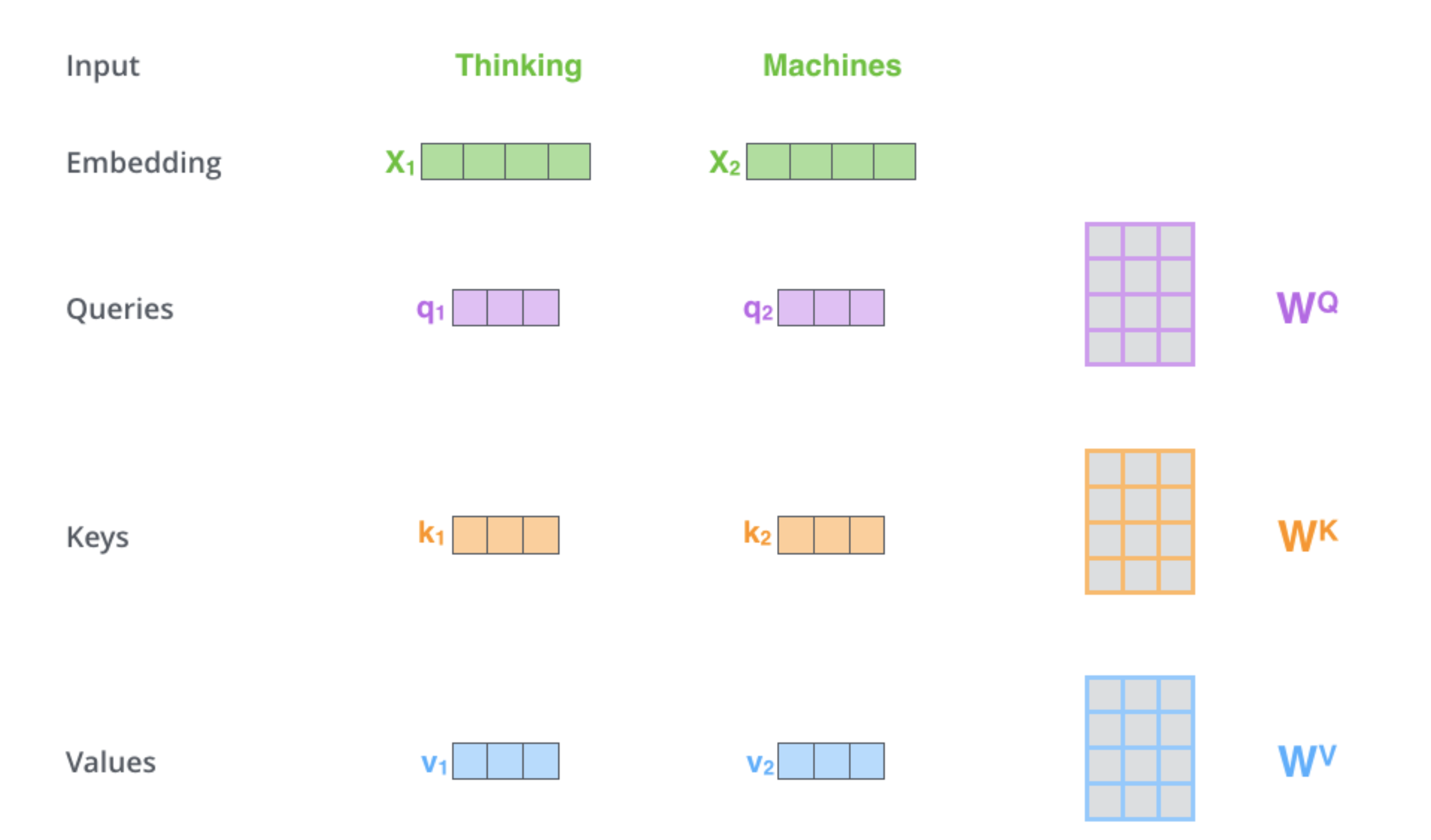
The first step is to project the input into 3 different vector spaces: key space, query space and value space. These projections give us a key vector, a query vector and a value vector. The weights of these projection matrices are learnt via backpropagation during training. The projection matrices for key, query and value are $W^{K}$, $W^{Q}$, $W^{V}$ respectively. These projections are exactly what we discussed above. Their values depend a lot on the training procedure and the training data.
-
The next step is to calculate attention scores. This is basically the part where we determine how similar are two input vectors and hence how much attention/focus needs to be paid on one vector while summarizing the other.
The score determines how much focus to place on other parts of the input sentence as we encode a word at a certain position.
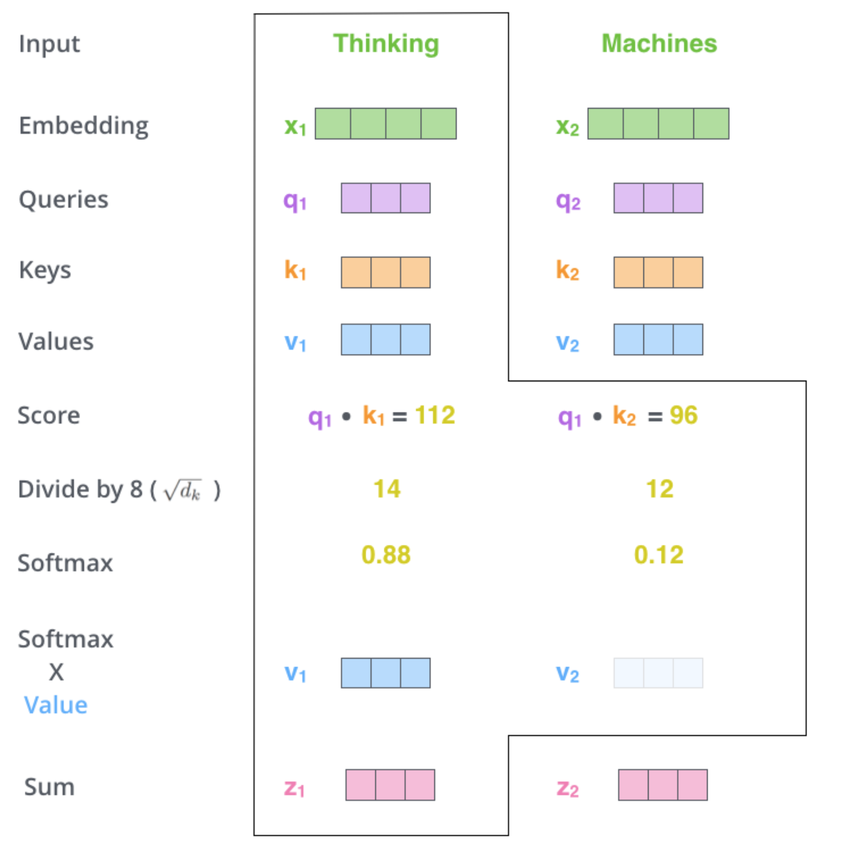
There are different ways to determine this. In this paper, a dot product between the query and the key is used. Consider the phrase "Thinking Machines". For the word "Thinking", we need to calculate a score with each word in the sentence including "Thinking" itself. Therefore, score for first position would be, $$ q_{1}\ .\ k_{1} $$ The result of this product represents the amount of attention we need to pay to "Thinking" itself while encoding "Thinking". The score for next position would be, $$ q_{1}\ .\ k_{2} $$ which captures the importance of "Machines" while encoding "Thinking".
- We then divide the scores calculated in the previous step by $\sqrt d_{k}$, where $d_{k}$ is the dimension of key vectors. This scaling was done to ensure that the gradients are stable during training. Next, these scores are passed through a softmax function to get an attention distribution. This means that for a sentence of length $n$, if $\alpha_{t}$ represents the score at $t$-th position, then $$ \sum_{t=1}^{n} \alpha_{t} = 1$$
- The last step is to multiply the softmax output with the value vector at respective position and sum these products up. In effect this computes a weighted sum. For a sentence of length n, $$ \sum_{t=1}^{n} \alpha_{t}\ v_{t}$$
All the steps explained above can be summarized as,
Multiheaded attention and Implementation
The above steps are usually performed using matrices instead of vectors. This is also where we'll see how and why multihead attention is implemented.
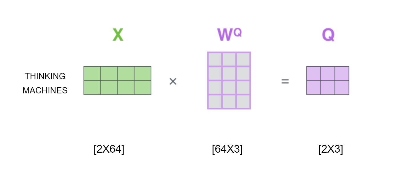
- The first step is to calculate the query, key and value matrices by projecting them using trainable weights. In code, these weights correspond to linear layers. $W^{Q}$ corresponds to
fc_q, $W^{K}$ tofc_kand $W^{V}$ tofc_v. Projecting these gives us $Q$, $K$ and $V$ as seen in code too.
- Calculation of scores can be easily visualized as follows,
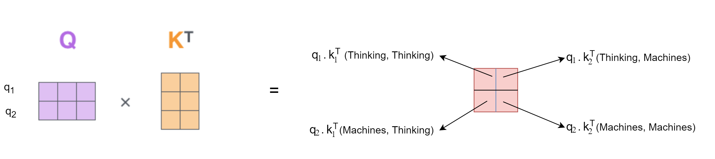
In code this is achieved by calculating theenergyof $K$ and $Q$ usingtorch.matmul. - The final step is to scale, take softmax of the scores and multiply the matrix by the value matrix.
scaleis calculated by taking the square root ofhead_dim. After scaling theenergytensor or the scores at different positions, we apply softmax to this tensor and multiply it with $V$ usingtorch.matmulonce again.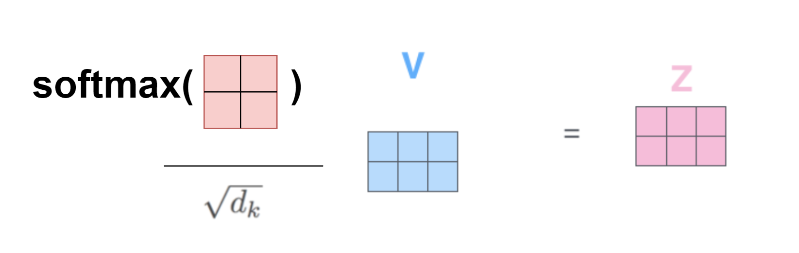
In the original transformer model, the input embedding size is 512. Before projecting these embeddings, we split them into 8 parts which brings us to multihead attention. This paper uses 8 attention heads.
Multiheaded attention expands the model's ability to focus on different positions.
It gives the attention layer mutiple "representation subspaces."
These subspaces are nothing but different projection matrices. Instead of having just one projection matrix $W^{Q}$ for query, we'll have 8 projection matrices for query, key and value. Weights for each of these "subspaces" are learnt via backpropagation during training. An analogy for this can be the use of multiple convolutional filters to learn unique features from the image.
Therefore, now the dimension of key, query and value matrices would be 64 (512/8). In code, splitting weight matrices for multiple attention heads is done right after getting $K$, $Q$ and $V$. This is done by first calculating the head_dimension and then splitting the tensors using the view function.
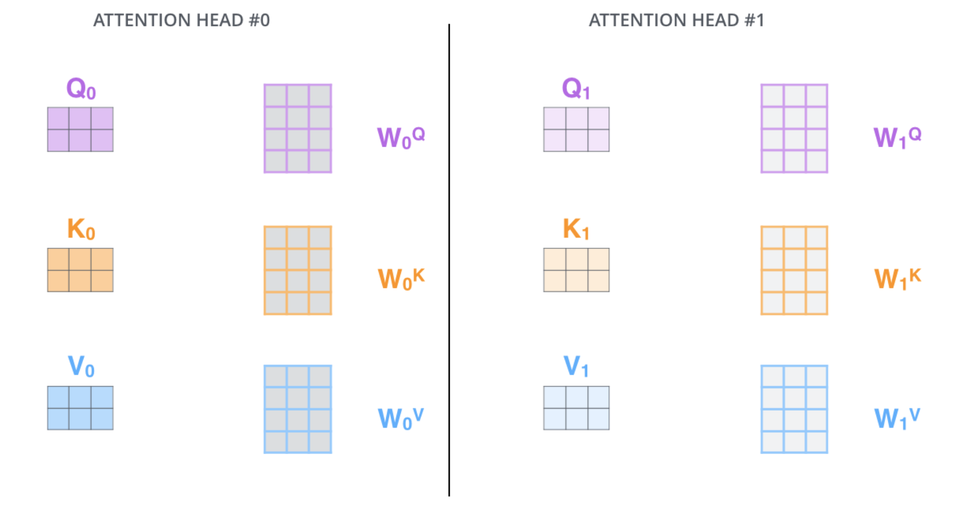
The above image shows projection matrices for 2 attention heads. There are 8 such heads. This would give us 8 $Z$ matrices in the end. The output dimension of the self attention layer should be same as the input dimension. Hence, we need to recombine the results of all the attention heads before passing the output to the next layer. To combine them, in code, we simply use view to drop the head dimension and further make a projection using fc_o to ensure that the input dimension is same as the output dimension.
from torch import nn

class MultiheadAttentionLayer(nn.Module):

    def __init__(self, hid_dim, num_heads, device):

        super().__init__()
        self.num_heads = num_heads
        self.device = device
        self.hid_dim = hid_dim

        self.head_dim = self.hid_dim // self.num_heads

        self.fc_q = nn.Linear(hid_dim, hid_dim)

        self.fc_k = nn.Linear(hid_dim, hid_dim)

        self.fc_v = nn.Linear(hid_dim, hid_dim)

        self.fc_o = nn.Linear(hid_dim, hid_dim)

        self.scale = torch.sqrt(torch.FloatTensor([self.head_dim])).to(device)


    def forward(self, x, mask):
        # x = [bs, len_x, hid_dim]
        # mask = [bs, len_x]

        batch_size = x.shape[0]

        Q = self.fc_q(x)
        K = self.fc_k(x)
        V = self.fc_v(x)
        # Q = K = V = [bs, len_x, hid_dim]

        Q = Q.view(batch_size, -1, self.num_heads, self.head_dim).permute(0,2,1,3)
        K = K.view(batch_size, -1, self.num_heads, self.head_dim).permute(0,2,1,3)
        V = V.view(batch_size, -1, self.num_heads, self.head_dim).permute(0,2,1,3)
        # [bs, len_x, num_heads, head_dim ]  => [bs, num_heads, len_x, head_dim]

        K = K.permute(0,1,3,2)
        # [bs, num_heads, head_dim, len_x]

        energy = torch.matmul(Q, K) / self.scale
        # (bs, num_heads){[len_x, head_dim] * [head_dim, len_x]} => [bs, num_heads, len_x, len_x]

        mask = mask.unsqueeze(1).unsqueeze(2)
        # [bs, 1, 1, len_x]

        #print("Mask: ", mask)
        #print("Energy: ", energy)

        energy = energy.masked_fill(mask == 1, -1e10)

        #print("energy after masking: ", energy)

        alpha = torch.softmax(energy, dim=-1)
        #  [bs, num_heads, len_x, len_x]

        #print("energy after smax: ", alpha)
        alpha = F.dropout(alpha, p=0.1)

        a = torch.matmul(alpha, V)
        # [bs, num_heads, len_x, head_dim]

        a = a.permute(0,2,1,3)
        # [bs, len_x, num_heads, hid_dim]

        a = a.contiguous().view(batch_size, -1, self.hid_dim)
        # [bs, len_x, hid_dim]

        a = self.fc_o(a)
        # [bs, len_x, hid_dim]

        #print("Multihead output: ", a.shape)
        return a
References
- Attention is All You Need https://papers.nips.cc/paper/7181-attention-is-all-you-need.pdf
- https://lilianweng.github.io/lil-log/2018/06/24/attention-attention.html
- The Illustrated Transformer:http://jalammar.github.io/illustrated-transformer/. This is an excellent piece of writing with amazing easy-to-understand visualizations. Must read.
- https://mccormickml.com/2019/11/11/bert-research-ep-1-key-concepts-and-sources/. Chris McCormick's BERT research series is another great resource to learn about self attention and various other details about BERT. He has a blog as well as youtube video series on the same.
- https://nlp.seas.harvard.edu/2018/04/03/attention.html. The annotated Transformer.
- https://web.stanford.edu/class/archive/cs/cs224n/cs224n.1184/lectures/lecture10.pdf.
- https://github.com/bentrevett/pytorch-seq2seq. A great series of notebooks on Machine Translation using PyTorch which includes all the the methods discussed above in greater detail and context.