Character Embeddings and Highway Layers in NLP
Understand in detail using code a repetitve pattern in many important NLP systems.


Introduction
Character embeddings and Highway Layers are the trademark components of many NLP systems. They have been used extensively in literature to reduce the parameters in models, deal with Out of Vocabulary or OOV words and help in faster training of neural networks. This blog post introduces these 2 topics, explains the intuitions with illustrations and then translates everything into code.
This blog post is a small excerpt from my work on paper-annotations for the task of question answering. This repo contains a collection of important question-answering papers, implemented from scratch in pytorch with detailed explanation of various concepts/components introduced in the respective papers.
Character Embedding
It maps each word to a vector space using character-level CNNs.
Using CNNs in NLP was first proposed by Yoon Kim in his paper titled Convolutional Neural Networks for Sentence Classification. This paper tries to use CNNs in NLP as they are used in vision. Most of the state-of-the-art results in CV at that time were achieved by transfer learning from larger models pretrained on ImageNet. In this paper, they train a simple CNN with one layer of convolution on top of pretrained word vectors and hypothesized that these pretrained word vectors could work as a universal feature extractors for various classification tasks. This is analogous to the earlier layers of vision models like VGG and Inception working as generic feature extractors. The idea of character embeddings was also used in the paper titled Character-Aware Neural Language Models by the same author. The intuition is simple over here. Just as convolutional filters learn various features in an image by operating on its pixels, here they'll do so by operating on characters of words. Let's get into the working of this layer.
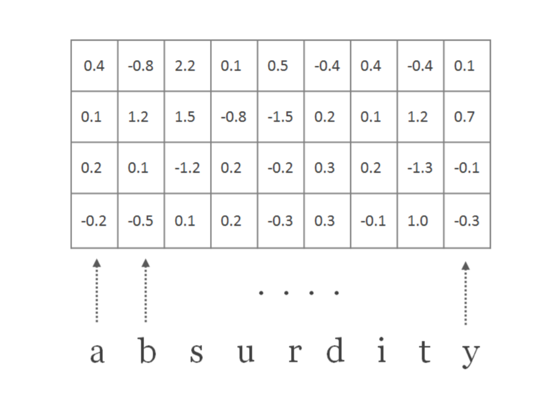
We first pass each word through an embedding layer to get a fixed size vector. Let the embedding dimension be $d$.
Let $C$ represent a matrix representation of word of length $l$. Therefore $C$ is a matrix with dimensions $d$ x $l$.
Let $H$ represent a convolutional filter with dimensions $d$ x $w$, where $d$ is the embedding dimension and $w$ is the width or the window size of the filter.
The weights of this filter are randomly initialized and learnt parallelly via backpropogation. We convolve this filter $H$ over our word representation $C$ as shown below.
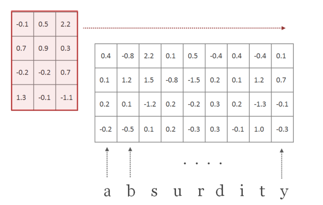
The convolution operation is simply the inner product of the filter $H$ and matrix $C$. The convolution operations can be visualized as follows:
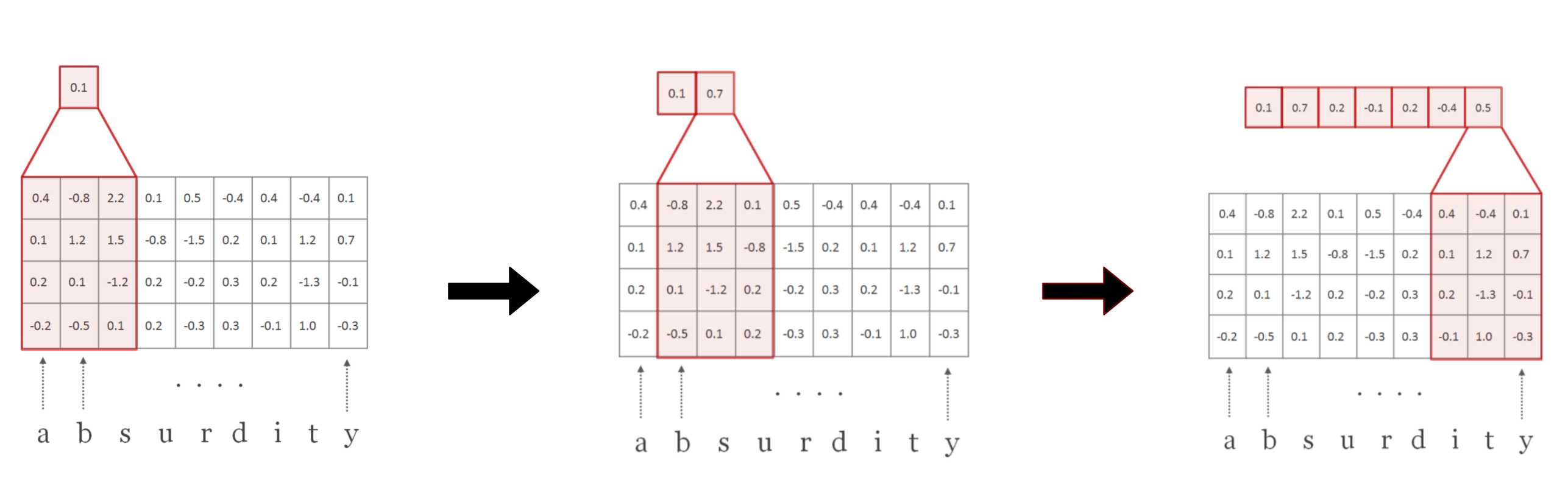
The result of the above operation is a feature vector. A single filter is usually associated with a unique feature that it captures from the image/matrix. To get the most representative value related to the feature, we perform max pooling over the dimension of this vector.
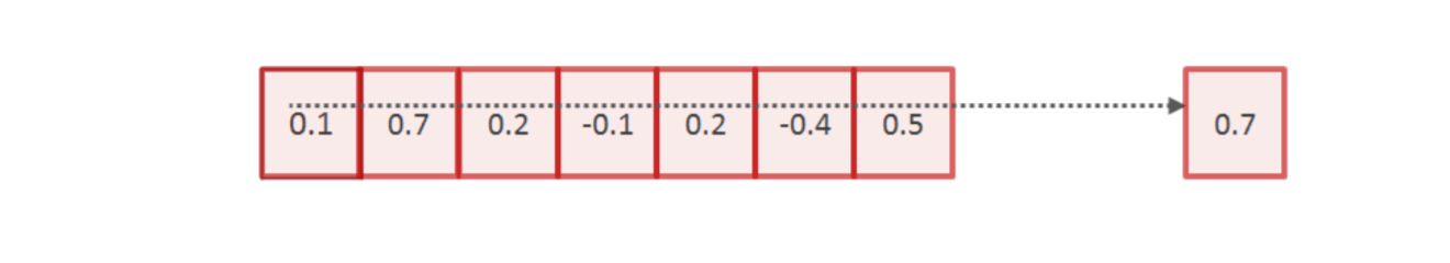
The above process was described for a single filter. This same process is repeated with $N$ number of filters. Each of these filters captures a different property of word. In an image, for example, if one filter captures the edges, another filter will capture the texture and another one the shapes in the image and so on. $N$ is also the size of the desired character embedding. In this paper authors have trained the model with $N$ = 100.
Implementation
The implementation of this layer is fairly straightforward. The input to this layer is of dimension [batch_size, seq_len, word_len] where seq_len and word_len are the lengths of largest sequence and word respectively within a given batch . We first embed the character tokens into a fixed size vector using an embedding layer. This gives a vector of dimension [batch_size, seq_len, word_len, emb_dim].
We then convert this tensor into a format that closely resembles an image, of type [ $N$, $C_{in}$, $H_{in}$, $W_{in}$]. The number of input channels, $C_{in}$ would be 1 and the output channels would be the desired embedding size which is 100. This is then passed through the convolution layer which gives an output of shape [ $N$, $C_{out}$, $H_{out}$, $W_{out}$]. Here,
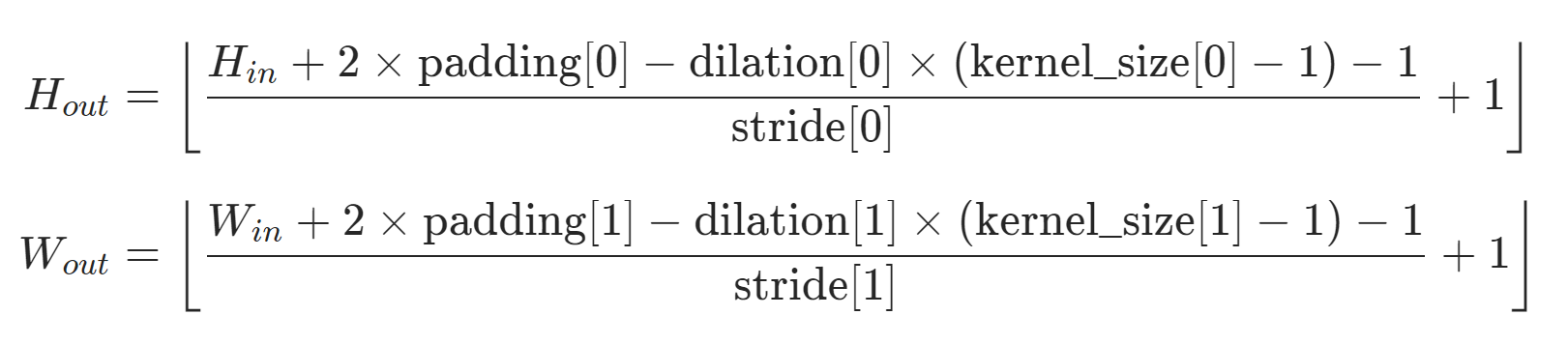
If padding = [0,0], kernel_size (or filter-size) = [$H_{in}$, $w$], dilation = [1,1], stride = [1,1].
as visible in images above, then,
$H_{out}$ = 1, and $W_{out}$ = $W_{in}$ - $w$ - 1.
Since $H_{out}$ = 1, we squeeze that dimension and perform max pooling with a kernel-size = $L_{in}$. The value of $L_{in}$ = $W_{in}$ - $w$ - 1.
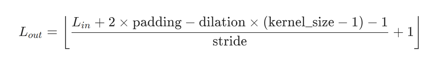
If the kernel size = $L_{in}$, we get $L_{out}$ = 1 if other values are default. This dimension is again squeezed to finally give us a tensor of dimension [batch_size, seq_len, output_channels (or 100)].
class CharacterEmbeddingLayer(nn.Module):

    def __init__(self, char_vocab_dim, char_emb_dim, num_output_channels, kernel_size):

        super().__init__()

        self.char_emb_dim = char_emb_dim

        self.char_embedding = nn.Embedding(char_vocab_dim, char_emb_dim, padding_idx=1)

        self.char_convolution = nn.Conv2d(in_channels=1, out_channels=100, kernel_size=kernel_size)

        self.relu = nn.ReLU()

        self.dropout = nn.Dropout(0.2)

    def forward(self, x):
        # x = [bs, seq_len, word_len]
        # returns : [batch_size, seq_len, num_output_channels]
        # the output can be thought of as another feature embedding of dim 100.

        batch_size = x.shape[0]

        x = self.dropout(self.char_embedding(x))
        # x = [bs, seq_len, word_len, char_emb_dim]

        # following three operations manipulate x in such a way that
        # it closely resembles an image. this format is important before
        # we perform convolution on the character embeddings.

        x = x.permute(0,1,3,2)
        # x = [bs, seq_len, char_emb_dim, word_len]

        x = x.view(-1, self.char_emb_dim, x.shape[3])
        # x = [bs*seq_len, char_emb_dim, word_len]

        x = x.unsqueeze(1)
        # x = [bs*seq_len, 1, char_emb_dim, word_len]

        # x is now in a format that can be accepted by a conv layer.
        # think of the tensor above in terms of an image of dimension
        # (N, C_in, H_in, W_in).

        x = self.relu(self.char_convolution(x))
        # x = [bs*seq_len, out_channels, H_out, W_out]

        x = x.squeeze()
        # x = [bs*seq_len, out_channels, W_out]

        x = F.max_pool1d(x, x.shape[2]).squeeze()
        # x = [bs*seq_len, out_channels, 1] => [bs*seq_len, out_channels]

        x = x.view(batch_size, -1, x.shape[-1])
        # x = [bs, seq_len, out_channels]
        # x = [bs, seq_len, features] = [bs, seq_len, 100]


        return x
Highway Networks
Highway networks were originally introduced to ease the training of deep neural networks. While researchers had cracked the code for optimizing shallow neural networks, training deep networks was still a challenging task owing to problems such as vanishing gradients etc. Quoting the paper,
We present a novel architecture that enables the optimization of networks with virtually arbitrary depth. This is accomplished through the use of a learned gating mechanism for regulating information flow which is inspired by Long Short Term Memory recurrent neural networks. Due to this gating mechanism, a neural network can have paths along which information can flow across several layers without attenuation. We call such paths information highways, and such networks highway networks.
This paper takes the key idea of learned gating mechanism from LSTMs which process information internally through a sequence of learned gates. The purpose of this layer is to learn to pass relevant information from the input. A highway network is a series of feed-forward or linear layers with a gating mechanism. The gating is implemented by using a sigmoid function which decides what amount of information should be transformed and what should be passed as it is.
A plain feed-forward layer is associated with a linear transform $H$ parameterized by ($W_{H}, b_{H}$), such that for input $x$, the output $y$ is
$$ y = g(W_{H}.x + b_{H})$$
where $g$ is a non-linear activation.
For highway networks, two additional linear transforms are defined viz. $T$ ($W_{T},b_{T}$) and $C$ ($W_{C}$,$b_{C}$).
Then,
$$ y = T(x) . H(x) + x . (1 - T(x)) $$ $$ y = T(x) . g(W_{H}.x + b_{H}) + x . (1 - T(x)) $$We refer to T as the transform gate and C as the carry gate, since they express how much of the output is produced by transforming the input and carrying it, respectively. For simplicity, in this paper we set C = 1 − T.
where $T(x)$ = $\sigma$ ($W_{T}$ . $x$ + $b_{T}$) and $g$ is relu activation.
The input to this layer is the concatenation of word and character embeddings of each word. To implement this we use nn.ModuleList to add multiple linear layers. This is done for the gate layer as well as for a normal linear transform. In code the flow_layer is the same as linear transform $H$ discussed above and gate_layer is $T$. In the forward method we loop through each layer and compute the output according to the highway equation described above.
The output of this layer for context is $X$ $\epsilon$ $R^{\ d \ X \ T}$ and for query is $Q$ $\epsilon$ $R^{\ d \ X \ J}$, where $d$ is hidden size of the LSTM, $T$ is the context length, $J$ is the query length.
Importance in NLP systems
The structure discussed so far is a recurring pattern in many NLP systems. Although this might be out of favor now with the advent of transformers and large pretrained language models, you will find this pattern in many NLP systems before transformers came into being. The idea behind this is that adding highway layers enables the network to make more efficient use of character embeddings. If a particular word is not found in the pretrained word vector vocabulary (OOV word), it will most likely be initialized with a zero vector. It then makes much more sense to look at the character embedding of that word rather than the word embedding. The soft gating mechanism in highway layers helps the model to achieve this.
class HighwayNetwork(nn.Module):

    def __init__(self, input_dim, num_layers=2):

        super().__init__()

        self.num_layers = num_layers

        self.flow_layer = nn.ModuleList([nn.Linear(input_dim, input_dim) for _ in range(num_layers)])
        self.gate_layer = nn.ModuleList([nn.Linear(input_dim, input_dim) for _ in range(num_layers)])

    def forward(self, x):

        for i in range(self.num_layers):

            flow_value = F.relu(self.flow_layer[i](x))
            gate_value = torch.sigmoid(self.gate_layer[i](x))

            x = gate_value * flow_value + (1-gate_value) * x

        return x
References
- Character-Aware Neural Language Models: https://arxiv.org/abs/1508.06615
- Convolutional Neural Networks for Sentence Classification: https://arxiv.org/abs/1408.5882
- Highway Networks: https://arxiv.org/abs/1505.00387
- https://nlp.seas.harvard.edu/slides/aaai16.pdf. A great resource for character embeddings. The figures in the character embedding section are taken from here.