Introduction

This blog is about my recent research on generative modeling, variational autoencoders (VAEs) and, in particular, application of VAEs to text generation. VAEs work extremely well for images but have not seen the same success in text-generation. This is because VAE training for such models usually results in the model choosing a local optimum where it learns to completely ignore the latent variable. This phenomenon is referred to as the posterior collapse in literature. This blog assumes familiarity with the basics of latent variable models and VAEs. There are a lot of great resources that explain the ideas and the math behind VAEs. I begin with a small recap of latent variable models, the evidence lower bound (ELBO) and how VAEs model the probability distibutions of the ELBO. I then move on to the application of VAE models for text generation, optimization challenges and their proposed solutions. To do this, I explain 2 papers related to the topic which look at the problem in unique ways and propose different solutions for the same. I hope that by the end of this blog, the reader gains a solid understanding of the basics, motivations, challenges and the proposed solutions for training text-generating VAEs.

Latent Variable Models and Variational Autoencoders

Any dataset for a given problem comprises of datapoints $x_{i}$'s. These datapoints are usually recorded as part of some data collection process or are simply generated as a byproduct of another process. For example, determining the average heights of people across different countries, weather predictions, classifying if a medical image shows a benign or a malignant tumor and so on. In all such cases, we would like to know more about the data generating process itself, rather than only having some samples of the process. However, this is not practically possible. Instead, we assume that the datapoints that we have come from some probability distribution and try to approximate it using the data. One can argue that by doing so, we are making a very strong assumption about the data coming from some well defined data generating process (probability distribution). But it would be very pessimistic to believe that everything is completely random. It would call for our nature being too dull (when we already know it is not) to not enforce some structure on the many happenings in our surroundings.
Latent variable models (LVMs) assume that an observed datapoint $x_{i}$ is generated by a latent variable $z$ which we cannot observe. These latent variables capture some interesting structure about the data which is not obvious. A graphical model for the above idea can be described as $$z \rightarrow x$$

Evidence Lower Bound

VAEs are a class of LVMs that optimize the evidence lower bound (ELBO) using variational inference in a way that scales well for large datasets. This can be attributed to the reparameterization trick which enables us to use gradient optimization methods like stochastic gradient descent to optimize the lower bound. The lower bound equation after applying reparameterization can be written as

$$L(\theta, \phi) = E_{q_{\phi}(z|x)}[\log p_{\theta}(\ x\ |\ z)] - KL\ [q_{\phi}(\ z\ |\ x\ ))\ ||\ p(z)]$$

For the VAE, we have following definitions and assumptions,

$p(z)$ is the prior which is taken a standard multivariate gaussian, with mean ($\mu$) = 0 and variance $(\sigma)$ = $I$.
$p_{\theta}(x\ |\ z)$ is a multivariate gaussian, parameterized by a neural net or a multi-layer perceptron (MLP). Given a multi-dimensional $z$, this MLP outputs the mean ($\mu_{\theta}$) and variance ($\sigma_{\theta}$) of the assumed gaussian.
$q_{\phi}(z\ |\ x)$ is the approximate posterior or the inference model that we use to estimate the true posterior $p_{\theta}(z\ |\ x)$. This is assumed to be a multivariate gaussian whose parameters are calculated by a neural net. It takes $x$ as input and outputs the mean ($\mu_{\phi}$) and the variance ($\sigma_{\phi}$) of the distribution.

It is easy to see that the approximate posterior $q_{\phi}(z\ |\ x)$ acts as an encoder taking in a datapoint $x$ and giving out a latent representation of the input, $z$. Similarly, $p_{\theta}(x\ |\ z)$ acts as the decoder in VAE, taking in the encoded latent variable and again reconstructing the input example, $x$.

$$x \xrightarrow{q_{\phi}(z\ |\ x)}\ z\ \xrightarrow{p_{\theta}(x\ |\ z)}\ x$$

VAE for Sentences

Language models assign probabilities to sequences of natural text and are used to predict the next best word based on previous context. The probability of a sequence with $m$ words can be modeled as,

$$ p(w_{1}, w_{2}... w_{m}) = \prod_{i=1}^{m}p(w_{i}\ |\ w_{1}, ...w_{i-1}) $$

The above equation can be simplified using some independence assumptions wherein we assume that the probability of next word does not depend on the entire sequence but only previous $n$ words. If $n=1$, we have a unigram language model, bigram if $n=2$ and so on. For a general n-gram model, we have the following approximation,

$$ \prod_{i=1}^{m}p(w_{i}\ |\ w_{1}, w_{2}... w_{i-1}) \approx \prod_{i=1}^{n}p(w_{i}|\ w_{i-(n-1)}, ...w_{i-1}) $$

Recurrent neural networks (RNNs) and its variants (LSTMs/GRUs) can model this factorization and work well for generating natural text. In fact, theoretically, RNNs can model any arbitrarily long and complex sequence representation without any independence assumptions mentioned above. They fail in practice however, due to a number of issues. Nevertheless, if RNNs work reasonably well, a natural argument would then be, why do we need latent variables to generate text?
One of the motivations behind this is controlled generation of text. RNNs generate text at word or token level. They take a new input at each time step and emit out the next word based on the current input and several past inputs. It records the information from previous tokens in a continuously evolving hidden state vector. By doing so, it breaks the model structure into a series of next-word predictions and fails to capture sentence-level features like topic, high-level syntax and semantics.
With VAE, we can use a latent variable to encode the latent space of sentences which captures interpretable high-level features and decode or generate words from that space.
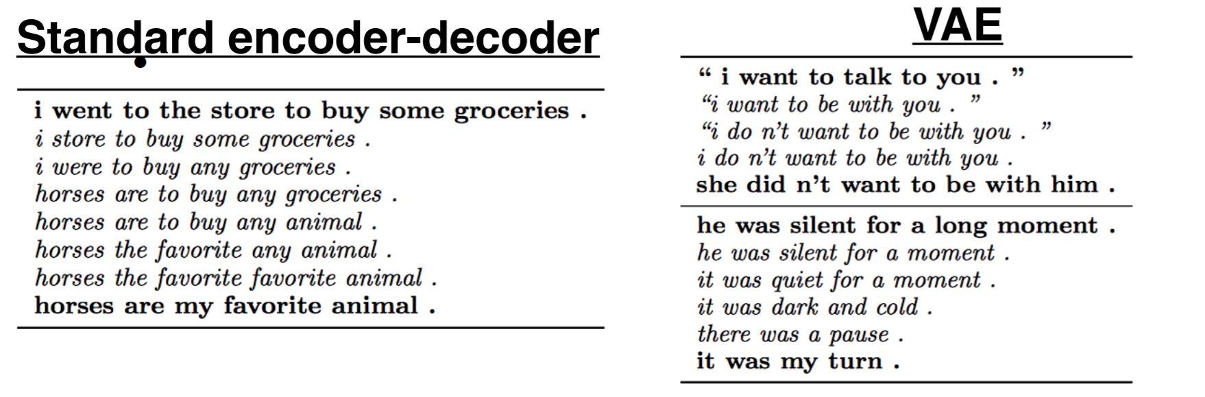
Following is an example that compares a standard encoder-decoder model and a VAE by interpolating vectors between two sentences (bold) vectors. We can see that halfway through, the standard model starts generating meaningless sentences because the decoding space for the model does not correspond to any reasonable semantics. Whereas, in case of the VAE, the intermediate sentences are semantically consistent.

Model

The model proposed by Bowman et al. is very similar in spirit to the original VAE. The only major difference is that the multivariate gaussians in the encoder and the decoder are parameterized by an LSTM model instead of a multi-layer perceptron. Like the VAE, they also use the reparameterization trick to enable backpropagation through the network. The proposed model can be explained by the figure below.

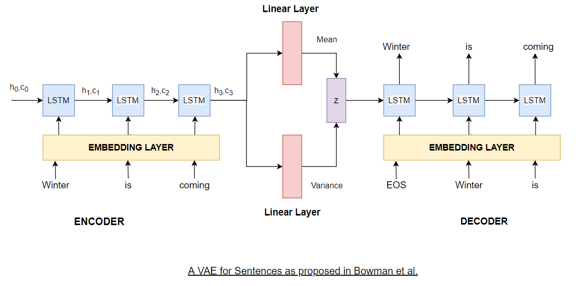
On the encoder side, we first get an embedding vector for each input token and pass it to an LSTM cell. We'll refer the tuple of hidden and cell state calculated by each LSTM unit as the hidden state for brevity. We use the hidden state vector of the final LSTM cell and consider it as the representation of the encoded sentence. This hidden state vector is then transformed by two linear layers, one to calculate the mean ($\mu_{\phi}$) and the other to calculate the variance ($\sigma_{\phi}$) of $q_{\phi}(z\ |\ x)$. The dimension of these linear layers is generally lesser than the hidden dimension of the LSTM cell. At this point, the reparameterization trick kicks in. To calculate $z$, we sample $\epsilon$ from a standard multivariate gaussian such that,

$$ \epsilon \sim \mathcal{N}(0, I)$$

$$ z = g_{\phi}(\epsilon, x) $$

$$ g_{\phi}(\epsilon, x) = \mu_{\phi}(x) + \epsilon \odot \sigma_{\phi}(x) $$

where $g_{\phi}$ is a differentiable transformation. By doing so, $z$ will also have the desired distribution as discussed earlier,

$$ q_{\phi}(z\ |\ x) \sim \mathcal{N}(z;\ \mu_{\phi}(x),\ \sigma_{\phi}(x))$$

Once we have the latent variable vector, we use it to initialize the hidden state of the first LSTM cell in the decoder. The input transformations in the decoder are similar to those in encoder. At each time-step we decode a word by passing the LSTM output at that time-step to a linear layer with softmax whose output dimension equals the vocabulary size. This is not generally shown in diagrams and is understood implicitly.

Optimization challenges

Training the model proposed above is not as straightforward as it seems. Training VAE models with very powerful decoders like RNNs/LSTMs is difficult because they suffer with posterior collapse. Posterior collapse occurs when the approximate posterior $q_{\phi}(z\ |\ x)$ equals (or collapses into) the prior $p(z)$. This means that the KL term in the lower bound optimization goes to zero and you're essentially only optimizing the cross-entropy loss of the decoder.

$$ L(\theta, \phi) = E_{q_{\phi}(z|x)}[\log p_{\theta}(\ x\ |\ z)] - KL\ [q_{\phi}(\ z\ |\ x\ ))\ ||\ p(z)] $$

$$ L(\theta, \phi) = E_{q_{\phi}(z|x)}[\log p_{\theta}(\ x\ |\ z)]\ if\ q_{\phi}(\ z\ |\ x\ ) = p(z) $$

This happens when the signal from the input $x$ to the posterior parameters is either too weak or too noisy. The decoder learns to ignore the information captured in the latent variable samples $z$ drawn from $q_{\phi}(z\ |\ x)$ altogether and results in very little signal passing from the encoder to the decoder. If the model learns to ignore $z$, the decoder is making predictions only based on the ground-truth inputs that we provide on the decoder side and is actually behaving as a general RNN language model (RNNLM). The decoding distribution can be described by the following equation,

$$ p(x\ |\ z) = \prod_{i}p(x_{i}\ |\ z,\ x_{<_{i}})$$

As discussed previously, the RNN based decoder does not need $z$ to optimize the lower bound because it can model any arbitrary sequential representation based on past inputs. It is also important to understand the dynamics of the lower bound equation which can be broken into 2 parts: the data likelihood under the posterior (expressed as cross entropy) and the KL divergence of the posterior from the prior. The cross-entropy term is a negative value since we're calculating the expectation of the log of a probability distribution (which lies between 0 and 1). The KL (which is always >=0) term is preceded with a negative sign which makes it negative too. Therefore the lower bound or the ELBO takes a negative value and maximizing it means that it should have a lower value.

So, technically, when the model suffers with posterior collapse, it is actually leading us to an easier optimization solution by making the KL term zero. But that kind of defeats the whole purpose of our premise! We do not want the model to learn only via the decoder. Instead we want the model to use the information captured in the latent variable to decode better representations that capture the high-level syntax and semantics of the text. Understanding the KL term can also be a bit counter-intuitive initially. The aim of the KL term is to drive the approximate posterior towards the prior, but that does not mean that we want them to be equal to each other. You can think of it as a regularization term.

Regularization is a technique used for tuning the function by adding an additional penalty term in the error function. The additional term controls the excessively fluctuating function such that the coefficients don’t take extreme values.

In our context, a model that encodes useful information in the latent variable $z$ should have a non-zero KL divergence and relatively small cross-entropy term. The cross-entropy term is reported as negative log-likelihood (NLL) for language modeling tasks in all the papers. A smaller cross-entropy term and a non-zero KL term would take care of all of our concerns. Hope is to capture enough useful information in the latent variable which helps the decoder to predict correctly and lower the cross-entropy term to a degree where even upon adding the non-zero KL term, it is still lesser than the local optimum attained via posterior collapse. $$ NLL + KL < NLL\ (with\ posterior\ collapse) $$

Proposed Solutions

There are two major categories of solutions to deal with posterior collapse in literature,

Alter the training procedure, wherein you change the training dyanmics to make sure that the latent variable is considered by the decoder while decoding.
Weaken the decoder, which means that we reduce information directly available to the decoder, such that it is forced to consider the latent variable $z$ for making decisions. There are many ways of doing this and some of them will be discussed below. Bowman et al. proposed the following solutions.

KL Cost Annealing

This technique can be put under the first catergory of solutions to deal with posterior collapse. The KL term is multiplied by a variable weight which is 0 during the initial stages of training. The weight is then increased progressively during training until it becomes 1 which is when it trains according to the normal VAE equation. Intuitively, not penalizing the KL term initially allows the encoder to pack as much information as possible into the latent variable $z$ for the decoder to use when we gradually begin penalizing KL.

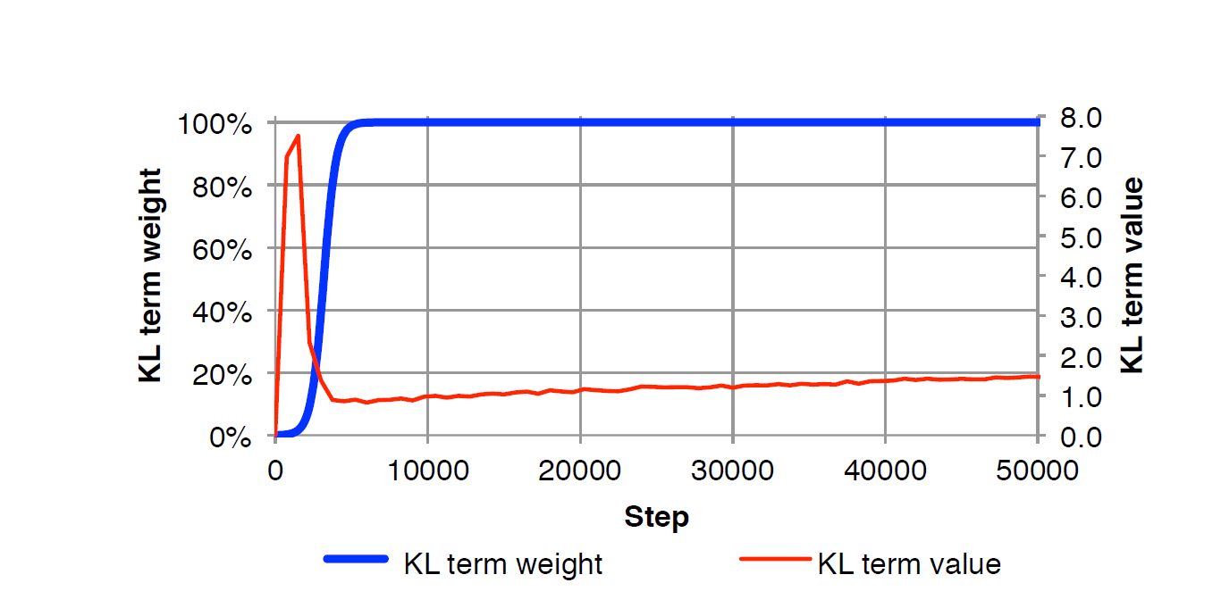
The graph above, taken directly from the paper summarizes the behaviour of the KL term and the variable weight. In the initial stages, when the variable weight is 0, the KL term spikes because the encoder, $q_{\phi}(z\ |\ x)$, can take in a lot of information without incurring any penalty. This drives $q_{\phi}(z\ |\ x)$ away from the prior, $p(z)$, hence the rise in KL. Then, as we gradually start increasing the variable weight, the value of KL term drops once the weight reaches 1. Finally, the KL term increases slowly as it converges and learns to pack information in $z$. The rate of increasing the variable weight is tuned as a hyperparameter.

Word Dropout

In vanilla dropout, we drop off some percentage of neurons from the neural network by setting the weights of these neurons as zero for that particular forward and backward pass. The idea behind dropout is to remove any dependencies between neurons and enable them to learn more robust features. It can also be thought of as a regularization technique since we are penalizing the model by not allowing it to use all the neurons and hence learn more complex features from the data. Word dropout proposed in Bowman et al. is similar in spirit. It is a way of weakening the decoder by reducing the information provided to the decoder directly. One way to implement this would be to dynamically update the embedding layer in the decoder. However, partially updating weights in an embedding layer during training is not as straightforward as it seems. Instead, word dropout is parameterized by a word keep rate $k\ \epsilon\ [0,1]$. At $k\ =\ 0$, the decoder has no inputs and predicts only based on the previously generated words and the latent variable $z$. The authors replace the ground-truth/label words with UNK tokens randomly which forces the decoder to look at the latent variable to predict the next word correctly. Intuitively, word dropout implements something that humans do quite naturally. If we already know about the text document we're going to read, we tend to skip a few words and are still able to make sense out of it. We're essentially relying on some latent information about the document within our brains, which is analogous to the idea behind word dropout.

Lagging Inference Networks

The paper discussed in this section by He et al. presents a different perspective of the posterior collapse as to why it happens and proposes a slightly altered training approach to avoid it. Unlike many other papers in literature, the authors specifically focus on the true model posterior $p_{\theta}(z\ |\ x)$ and the approximate posterior $q_{\phi}(z\ |\ x)$ and analyze how does their interaction throughout the training process determines whether the model will suffer with posterior collapse. The approximate posterior, $q_{\phi}(z\ |\ x)$ (also referred to as the inference network in this paper) is used to estimate the true posterior and hence the lower bound optimization tries to drive $q_{\phi}(z\ |\ x)$ towards $p_{\theta}(z\ |\ x)$. The authors hypothesize that during the initial stages of training, the inference network or $q_{\phi}(z\ |\ x)$ falls behind the true posterior (which it is supposed to approximate) which has multiple forces acting on it within the context of training dynamics. And before $q_{\phi}(z\ |\ x)$ can catch up with $p_{\theta}(z\ |\ x)$, the model learns to ignore $z$ and falls into a local optimum suffering with posterior collapse. We'll be going over the details of the core ideas in this paper.

Breaking down Posterior Collapse

Until now we have only discussed about the approximate posterior, $q_{\phi}(z\ |\ x)$ and prior $p(z)$ in the context of posterior collapse. However, the true model posterior, $p_{\theta}(z\ |\ x)$ also plays a key role in it, which the authors try to analyze and understand through various experiments. Formally, posterior collapse occurs when,

$$p_{\theta}(z\ |\ x)\ =\ q_{\phi}(z\ |\ x)\ =\ p(z)$$

We can further break posterior collapse into two partial collapse states,

Model collapse, when $p_{\theta}(z\ |\ x)\ =\ p(z)$
Inference collapse, when $q_{\phi}(z\ |\ x)\ =\ p(z)$

To conduct experiments and analyze the dynamics of the lower bound optimization, He et al. use a synthetic dataset, which is sequential in nature. They use an LSTM encoder and decoder since posterior collapse is more severe for such powerful autoregressive models.
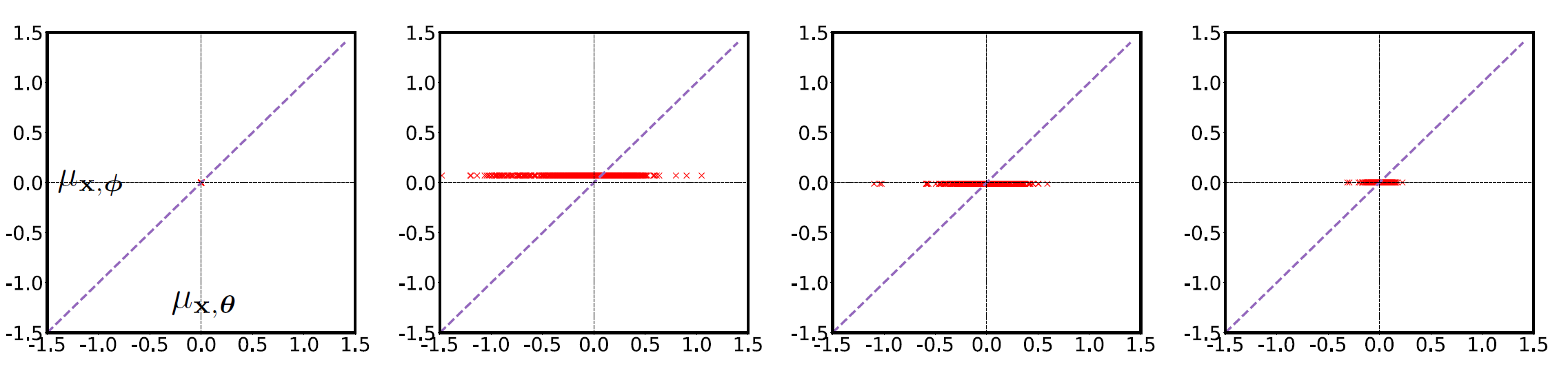
In order to observe how the true and approximate posterior change throughout the training process, we will keep track of their means. We have already discussed how we use neural networks to model multivariate gaussians. We will denote the true model posterior mean by $\mu_{x,\ \theta}$ and that of the inference network by $\mu_{x,\ \phi}$. The latent variable $z$ used in the experiments is a scalar, which will make it easier to visualize how these means change during training. Following figure, taken directly from the paper puts the above discussion into context.

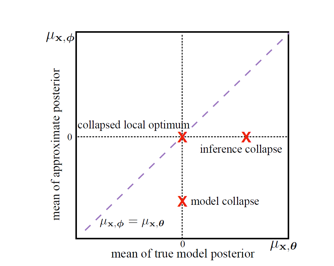
The figure highlights the following,

The x-axis denotes the mean $\mu_{x,\ \theta}$ of true model posterior, $p_{\theta}(z\ |\ x)$.
The y-axis denotes the mean $\mu_{x,\ \phi}$, of inference network $q_{\phi}(z\ |\ x)$
If the co-ordinates ( $\mu_{x,\ \theta}$, $\mu_{x,\ \phi}$) lie on x-axis, it means that the model has suffered with inference collapse because on x-axis, $\mu_{x,\ \phi}$ = 0, which is the mean of our prior, $p(z)$.
Similarly, if the co-ordinates ( $\mu_{x,\ \theta}$, $\mu_{x,\ \phi}$) lie on y-axis, it means that the model has suffered with model collapse because on x-axis, $\mu_{x,\ \theta}$ = 0, which is the mean of our prior, $p(z)$.
At the origin, we have posterior collapse where both the means collapse into 0.
And finally, we have the line $x\ =\ y$. If the datapoints are distributed along this line, we would have a attained a more desirable local optmimum as compared to the trivial one at the origin. If the approximate posterior has a non-zero value, it implies that the model has captured some useful information in the latent variable which will be used by the decoder.
NOTE It is not possible to calculate the true model posterior since it involves an intractable integral. The authors approximate the true model posterior by using a descretization method.

Visualizing Posterior Collapse

In this section, we'll be discussing the training dynamics of an alternate lower bound equation and analyze why do models suffer with posterior collapse. We can derive this alternate lower bound by looking at another optimization problem. We know that the evaluating true model posterior involves an intractable integral. Hence we try to approximate it using another probability distribution, $q_{\phi}(z\ |\ x)$. Our aim is to drive this towards the true model posterior and essentially we need to minimize the difference between these two distributions.

$$\min_{\phi,\ \theta}\ KL\ [q_{\phi}(z\ |\ x)\ ||\ p_{\theta}(z\ |\ x)]$$

$$KL\ [q_{\phi}(z\ |\ x)\ ||\ p_{\theta}(z\ |\ x)] = \int_{z} q_{\phi}(z\ |\ x)\ log \frac{q_{\phi}(z\ |\ x)}{p_{\theta}(z\ |\ x)}$$

$$KL\ [q_{\phi}(z\ |\ x)\ ||\ p_{\theta}(z\ |\ x)]\ =\ \int_{z} q_{\phi}(z\ |\ x)\ log \frac{q_{\phi}(z\ |\ x)\ p_{\theta}(x)}{p_{\theta}(z\ ,\ x)}$$

$$ KL\ [q_{\phi}(z\ |\ x)\ ||\ p_{\theta}(z\ |\ x)]\ =\ \int_{z} q_{\phi}(z\ |\ x)\ log \frac{q_{\phi}(z\ |\ x)}{p_{\theta}(z\ ,\ x)}\ +\ \int_{z} q_{\phi}(z\ |\ x)\ log\ p_{\theta}(x)$$

$$KL\ [q_{\phi}(z\ |\ x)\ ||\ p_{\theta}(z\ |\ x)]\ =\ -L(\theta, \phi) + log\ p_{\theta}(x)$$

Rearranging the above equation, we get the final ELBO as,

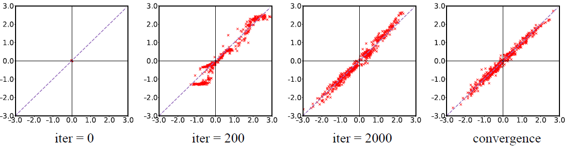
$$\boxed{L(\theta, \phi) = log(\ p_{\theta}(x)\ ) - KL\ [q_{\phi}(z\ |\ x)\ ||\ p_{\theta}(z\ |\ x)]}$$

According this equation, during training, there is only one force acting on $q_{\phi}(z\ |\ x)$ which is the KL term trying to drive it towards $p_{\theta}(z\ |\ x)$. However, there are two forces affecting the true posterior: the KL term and the marginal data likelihood. The following figures show what happens during different stages of training. These are the projections of 500 data samples generated from a synthetic dataset.

During the initial stages of training, $x$ and $z$ are independent under both $p_{\theta}(z\ |\ x)$ and $q_{\phi}(z\ |\ x)$. As shown in the figure at iter = 0, both the means are at 0 and since training has not begun yet, we say that all the datapoints are suffering with model collapse and inference collapse. As we start training, at around 200 iterations, the datapoints start spreading around the x-axis. Since $x$ and $z$ are independent under $p_{\theta}(z\ |\ x)$, the only remaining force acting on it is by the marginal data likelihood term. Hence, we can claim that $log\ p_{\theta}(x)$ is able to move the datapoints away from model collapse. However, if the datapoints are moving away from model collapse, that is $\mu_{x,\theta}$ is not zero anymore, it means that our true model posterior has changed via $log\ p_{\theta}(x)$. If the true model posterior changes, it implies that $p_{\theta}(z\ |\ x)$ will start diverging from $q_{\phi}(z\ |\ x)$ and therefore increase the KL term. $q_{\phi}(z\ |\ x)$ cannot keep track of this because $x$ and $z$ are still independent under it. Even under $p_{\theta}(z\ |\ x)$, the dependence is brought by $log\ p_{\theta}(x)$. So, even though the datapoints initially move away from model collapse, they are still in the state of inference collapse. As training progresses, datapoints are again brought close to 0 by an increasing KL term, which is evident at iter = 2000 in the figure above. The training process, thus makes an effort to align the true model posterior and the inference network by setting both to the prior $p(z)$. Before $q_{\phi}(z\ |\ x)$ can catch up with $p_{\theta}(z\ |\ x)$, the model has already learned to ignore the latent variable forcing the model into posterior collapse.

Relation with KL Cost Annealing

If we now take a step back and analyze KL cost annealing discussed earlier, we can clearly see why it actually works. In KL annealing, we do not penalize the KL term during the initial stages of training and start penalizing it gradually as training progresses. We can directly relate this to the ideas presented in the previous section. During the initial stages of training, we saw that the marginal data likelihood manages to move the datapoints away from model collapse. However, this is suppressed by an increasing KL term. The KL term rises because $p_{\theta}(z\ |\ x)$ diverges from $q_{\phi}(z\ |\ x)$ which is lagging behind the true model posterior. So even before $x$ and $z$ become dependent under $q_{\phi}(z\ |\ x)$, training forces the model into posterior collapse. We need to control the KL term in a way such that it waits for $q_{\phi}(z\ |\ x)$ to become relevant. This is exactly what KL annealing does. It essentially buys time for $q_{\phi}(z\ |\ x)$ to cover the lag and catch up with the true posterior by not penalizing the KL term initially.

Aggressive Training of the Inference Network

The solution proposed by He et al. is also intuitive. Since the inference network is lagging behind during the initial stages of training, we should optimize it before we optimize the true model posterior. Formally, this can be written as,

$$\theta^{*} =\ arg\max_{\theta}\ L(X; \theta, \phi^{*}),\ where\ \phi^{*} =\ arg\max_{\phi} L(X; \theta, \phi)$$

Essentially, it means that we're optimizing $q_{\phi}(z\ |\ x)$ in an inner loop in the entire training process. Also, the model need not operate in this mode throughout the training process. We need to do this only until $z$ and $x$ become dependent under $q_{\phi}(z\ |\ x)$ and it catches up with the true model posterior. Empirical results show that we typically need to train in aggessive mode for 5 epochs and then revert to normal training.

The figure above shows the behaviour posterior means when trained following the proposed aggressive training approach. The aggressive training successfully pulls the datapoints away from inference collapse and moves them towards the desired diagonal.

Closing Remarks

This blog covers some of the key ideas in this research area and I hope it gives the reader a solid foundation to build upon. I'll list down some other interesting ideas and papers in this topic that build upon the content presented in this blog. As discussed in the blog, most of the ideas to avoid posterior collapse can be broadly categorized under two categories: one that alters the training procedure and one that weakens/changes the decoder.

Improved Variational Autoencoders for Text Modeling using Dilated Convolutions

by Yang et al. replaces the recurrent decoder with a decoder which involves dilated convolutions. Dilated convolutions enable the network to increase the receptive field without incurring additional computations. In 2D convolution with different dilation $d$ can be visualized as follows

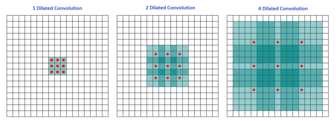
As can be see, for $d = 1$, the receptive field is $3X3$, for $d=2$, it is $7X7$ and for $d=4$, it is $15X15$. In all these convolutions the filter size effectively remains the same since we are skipping pixels in between. This idea translates to 1D and NLP applications in a similar fashion.

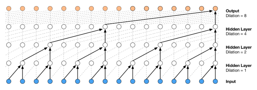
The authors hypothesize that there is a trade-off between contextual capacity of the decoder and effective use of encoding information. By changing the dilation structure of the decoder, we can control the contextual information from previously generated words. In extreme cases, the convolution decoder can act as a recurrent decoder (with less or no dilation) or as a simple MLP/bag-of-words model (with a big dilation factor). As such, we have a greater control over the amount of information provided to decoder via inputs. This can be thought of as a knob which allows us to change the complexity of the decoder from an LSTM to an MLP. LSTM decoders are strong enough to model an autoregressive factorization without using latent information. Hence, the authors believe that finding a sweet spot by turning this knob could lead us to better results which can take the advantage of both the latent and contextual information.

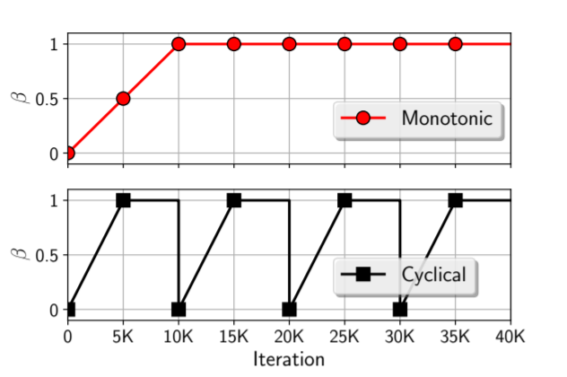
Cyclical Annealing Schedule: A Simple Approach to Mitigating KL Vanishing

by Fu et al. proposes a different KL annealing strategy. The authors argue against the de facto monotonic (Bowman et al.) KL annealing schedule and propose a cyclic schedule. Their hypothesis is based on analyzing the quality of latent variable $z$ learnt by the encoder during the initial stages of training.

References and Acknowledgements

I would like to thank Akash Srivastava, Swapneel Mehta and Fenil Doshi for introducing me to generative modeling and VAEs and clearing my doubts on numerous occasions. I would also like to thank Kumar Shridhar for clearing my doubts related to this research topic and suggesting edits to some sections of this blog. Below is the list of papers and other resources that I referred to while learning about this research area and writing this blog. Most of the figures in this blog have been borrowed from the concerned paper itself or some other blog, all of which have been mentioned in the references below and some were created by me using https://www.diagrams.net/. If you find any mistakes or errors, kindly point it out in the comments below or reach out to me at kushalj001@gmail.com. Thank you!