Introduction

Why another blog post on LSTMs?

LSTMs or the Long Short Term Memory have been around for a long time and there are many resources that do a great job in explaining the concept and its working in detail. So why another blog post? Multiple reasons. First, as a personal resource. I have read many blog posts on LSTMs and most of the times the same ones simply because I tend to forget the details after sometime. Clearly, my brain cannot handle long-term dependencies. Second, I am trying to put a lot of details in this post. I have come across blogs that explain LSTMs with the help of equations, some do it with text only and some with animations (hands down the best ones). In this post, I have attempted to include explanations for each component, equations, figures and an implementation of the LSTM layer from scratch. I hope this helps everyone get a wholesome understanding of the topic.

Recurrent Neural Nets

RNNs are one of the key flavours of deep neural networks. Unlike artificial neural networks that have multiple layers of neurons stacked one after another, it is not easily evident as to how recurrent nets are deep. Below is the figure of a rolled RNN.

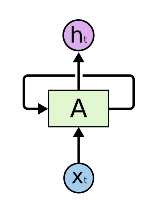
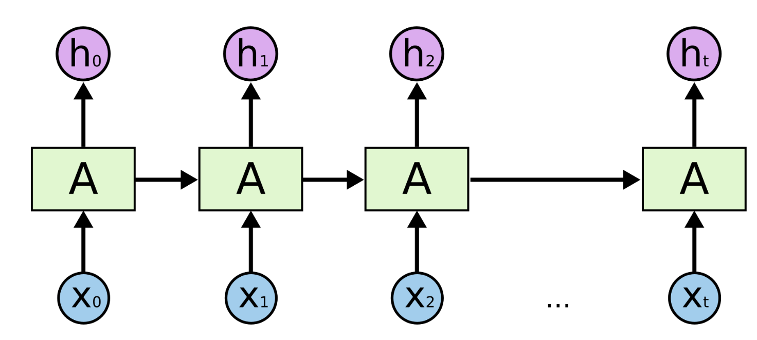
The input $x_{t}$ is processed by the RNN for each time-step t and outputs a hidden state that captures and maintains the information of all the previous time-steps. We'll see this again as a for loop when we implement an LSTM layer. This for loop is exactly what makes RNNs deep. The unrolled version of the network is more widely used in literature and is shown below:

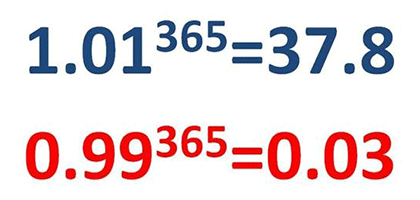
This deep nature is precisely the reason why such networks cannot practically model long-term dependencies. As the length of the input sequence increases, the number of matrix multiplications within the network increase. The weight updates of the earlier layers suffer as the gradients tend to vanish for them. Intuitively, think of this as multiplying a number less than zero with itself. The values become low exponentially. On the other hand if gradient values are larger than 1, these explode into large numbers that the computer can no longer make sense of. Consider this for intuition:

To deal with such issues, we need a mechanism that enables the networks to forget the irrelevant information and hold on to the relevant one. Enter LSTMs.

Understanding the LSTM cell

Before we get into the abstract details of the LSTM, it is important to understand what the black box actually contains. The LSTM cell is nothing but a pack of 3-4 mini neural networks. These networks are comprised of linear layers that are parameterized by weight matrices and biases. The values of these weights are learnt by backpropagation. The following figure shows an LSTM cell with labelled gates and all the computations that take place inside the cell. Each cell has 3 inputs: the current token $x_{t}$, previous hidden state $h_{t-1}$ and the previous cell state $c_{t-1}$ and 2 outputs: the updated hidden state $h_{t}$ and cell state $c_{t}$.

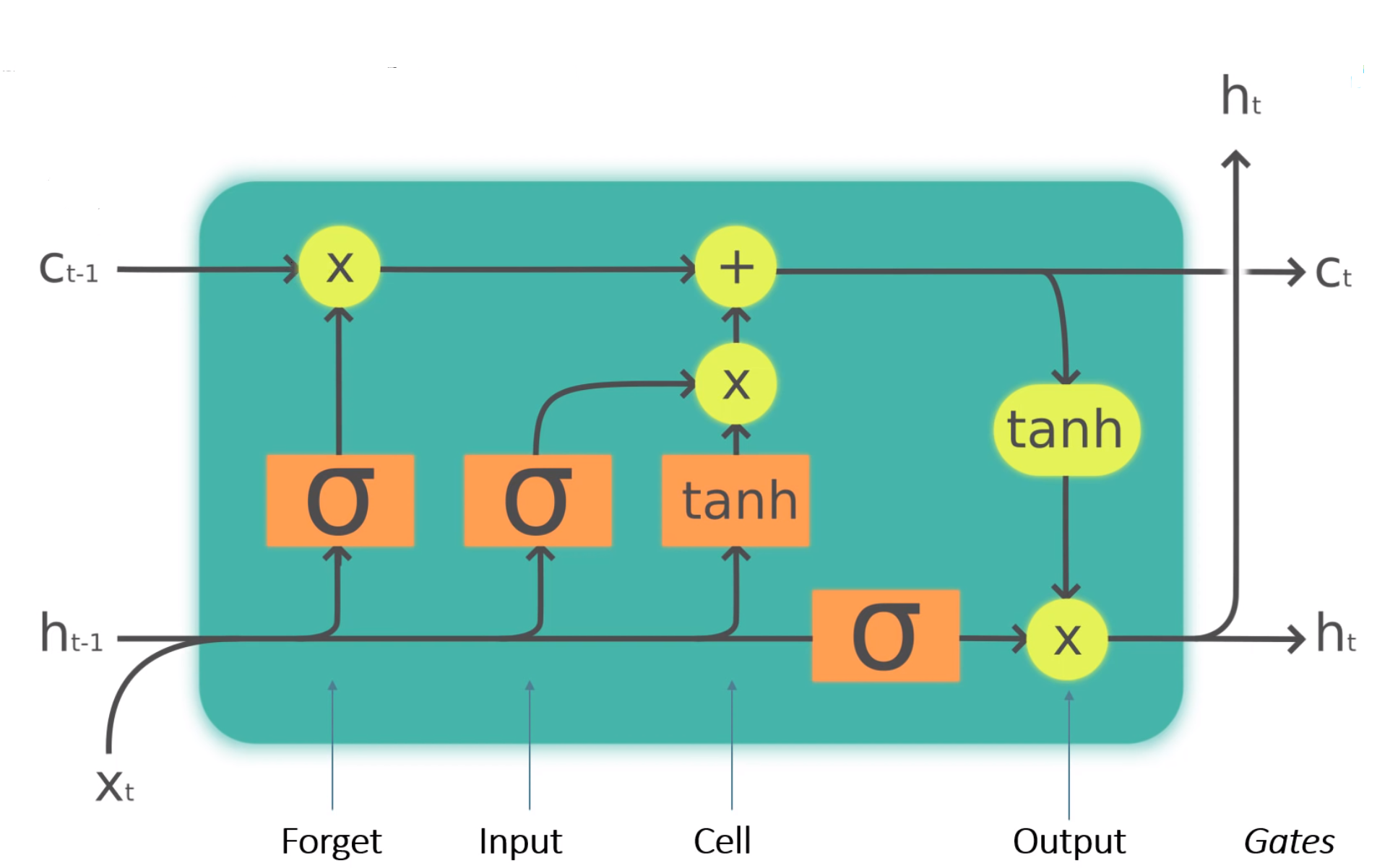
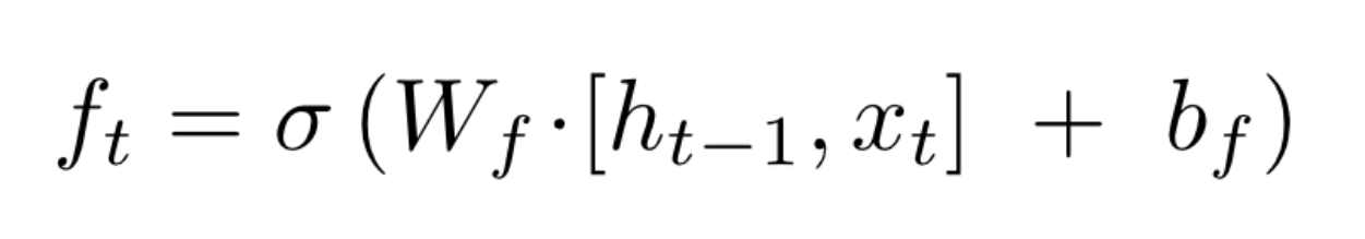
The forget gate

This gate takes in the current input $x_{t}$ and the previous hidden state $h_{t-1}$, multiplies them with a weight matrix of the forget gate $W_{f}$ (also adds a bias $b_{f}$) and applies a sigmoid activation. From an implementational point of view, $W_{f}$ and $b_{f}$ are the values associated with a simple linear layer. The sigmoid function restricts the input values between 0 and 1. This output is then multiplied with the cell state. Intuitively, given the current input this gate tells the cell to remove or forget some information if the sigmoid output is close to 0 and keep the information if the sigmoid output is close to 1. The equation for this gate is:

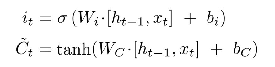
The input and the cell gate

The input gate is used to decide that given the current input what information is important and should be stored in the cell state. The calculations of this gate are similar to those of the forget gate. The cell gate and the input gate work closely together to perform a very specific function. This function is to update the previous cell state. To do so, the cell gate proposes an update candidate. You can think of this update candidate as a proposed new cell state. To calculate the cell gate output, a tanh activation is used (more on this later). The equation for the cell state is:

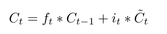
Cell update

We cannot simply replace the new proposed cell state and eliminate the previous cell state. This is because the previous state might contain some important information about the previous inputs the LSTM layer has seen. This is basically the main purpose of recurrent networks - to hold on to relevant information from the past. Hence, we adopt a very elegant approach to update the cell state.
From the previous blocks, we know the following:
Given the current input, the forget gate decides what information from the previous cell state can be forgotten. This is done by multiplying the forget gate output $f_{t}$ with the previous cell state $c_{t-1}$. Also, the input gate determines what information from the current input is relevant. Product of $i_{t}$ and the proposed cell state would give us important parts from the proposed cell state. We thus combine these two to yeild the following cell update equation:

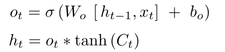
Output gate

This gate is used to calculate the hidden state for the next time step. Again the current input $x_{t}$ and previous hidden state $h_{t-1}$ are multiplied by a weight matrix $W_{o}$ and passed through sigmoid activation. To update the hidden state of the cell, it might be a good idea to incorporate some information from the newly updated cell state. Therefore, the result of the output gate $o_{t}$ is multiplied with the updated cell state $c_{t}$ after passing $c_{t}$ through tanh activation (explained later). The equation for this gate is:

Why do we use tanh for calculating cell state?

We left this part rather abruptly while talking about the cell gate. The question of as to why tanh has been preferred over sigmoid and even ReLU has been a hotly debated one. My research led me to multiple sources and reasons.

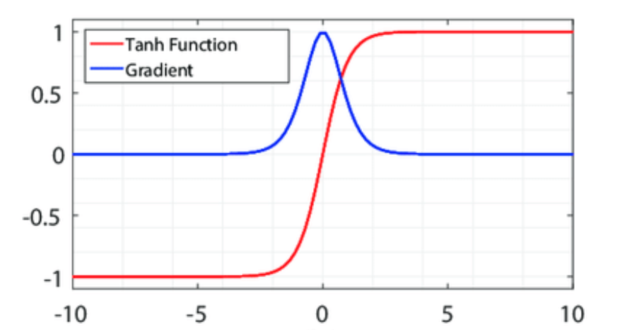
One of the key reasons as to why tanh is preferred is its range [-1, 1] and the fact that it is zero-centered. These properties enable the neural net to converge faster and hence train faster. Yann LeCun in his paper called Efficient BackProp explains such factors that affect the backpropagation algorithm in neural networks. To understand this consider the following. Assume that all the values in a weight matrix are positive. These weights are updated during backprop by say a factor d which can be positive or negative. As a result, these weights can only all decrease or all increase together for a given input pattern. Thus, if a weight vector must change direction it can only do so by zigzagging which is inefficient and thus very slow.
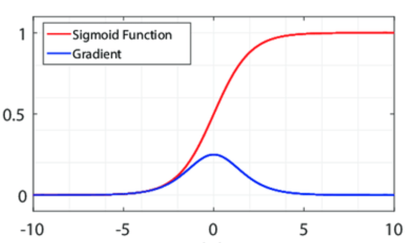
Another reason for using tanh is the relatively larger value of its derivative. Backprop computations result in multiplication of derivatives of the activation function multiple times depending upon the number of layers in the network. The maximum value for the derivative of a sigmoid function is 0.25 whereas that for tanh is 1. Hence, if the network is reasonably deep, the gradients of sigmoid are more likely to vanish than those of tanh.

For sigmoid the graph is

Why do we use tanh while calculating output gate values?

Although this is not that important but in case this question comes to your head, here's the answer. If you carefully look at the cell update equations, we have already applied a tanh activation in order to calculate the cell update candidate. Yet we again pass the cell state through tanh to get the new hidden state $h_{t}$. This is done to ensure that the values of $h_{t}$ lie between -1 and 1 because there's a chance that the values of the updated cell state $c_{t}$ might have exceeded 1 in previous additive computation.

Implementation

As pointed out earlier, the LSTM cell is a collection of 4 neural nets. In order to parallelize our computations and make use of a GPU it is better to compute values of the gates all at once. We need to linear layers: one for the current input and one for the previous hidden state.
So in the init method we initialize two linear layers. The out_features value for both these layers is 4 * hidden_dim owing to the number of gates.
You can relate this implementation with the equations above by expanding the multiplication of weights with the inputs. Assume that the weights associated with these layers are $W'_{i}$ for current input and $W'_{h}$ for previous hidden state. We perform the following computation initially and then break this computation into 4 matrices, one for each gate.

W = $W'_{i}$ $*$ $x_{t}$ + $W'_{h}$ $*$ $h_{t-1}$ + $b'_{i}$ + $b'_{h}$

The W matrix gets divided into 4 equal tensors $W_{i}$, $W_{f}$, $W_{c}$, $W_{o}$ which have been used in the equations above. This split is performed using torch.chunk.

The rest of the code for LSTM cell is just converting the equations to code.

import torch
from torch import nn

class LSTMCell(nn.Module):
    
    def __init__(self, input_dim, hidden_dim):
        
        super().__init__()
        self.input_layer = nn.Linear(in_features=input_dim, out_features=4 * hidden_dim)
        self.hidden_layer = nn.Linear(in_features=hidden_dim, out_features=4 * hidden_dim)
        
    def forward(self, current_input, previous_state):
        
        previous_hidden_state, previous_cell_state = previous_state
        
        weights = self.input_layer(current_input) + self.hidden_layer(previous_hidden)
        
        gates = weights.chunk(4,1)
    
        input_gate = torch.sigmoid(gates[0])
        forget_gate = torch.sigmoid(gates[1])
        output_gate = torch.sigmoid(gates[2])

        cell_gate = torch.tanh(gates[3])
        
        new_cell = (forget_gate * previous_cell_state) + (input_gate * cell_gate)
        new_hidden = output_gate * torch.tanh(new_cell)
        
        return new_hidden, (new_hidden, new_cell)

The following snippet basically takes an LSTMCell instance and calculates the output for the input sequence by applying a for loop. This is the same loop we had talked about initially in the post.

class LSTMLayer(nn.Module):
    
    def __init__(self, cell, *cell_args):
        
        super().__init__()
        self.cell = cell(*cell_args)
    
    def forward(self, input, state):
        
        inputs = input.unbind(1)
        outputs = []
        for i in range(len(inputs)):
            output, state = self.cell(inputs[i], state)
            outputs += [output]
        
        return torch.stack(outputs, dim=1), state

lstm = LSTMLayer(LSTMCell, 100, 100)

Acknowledgements and References

This blog post is merely a combination of a variety of great resources available on the internet. The code is heavily drawn from the fastai foundations notebook by Jeremy Howard who does a great job in explaining the inner workings of each component. Figures are majorly taken from Chris Olah's evergreen post on LSTMs. All the references and links have been listed below to the best of my knowledge. Thank you!