Building Sequential Models in PyTorch
Build a sentiment analysis model using PyTorch and torchText


- Introduction
- A short Introduction to NLP pipeline
- TorchText basics
- Implementing the model
- Training the model
- References and Acknowledgements
Introduction
The aim of this post is to enable beginners to get started with building sequential models in PyTorch. PyTorch is one of the most widely used deep learning libraries and is an extremely popular choice among researchers due to the amount of control it provides to its users and its pythonic layout. I am writing this primarily as a resource that I can refer to in future. This post will help in brushing up all the basics of PyTorch and also provide a detailed explanation of how to use some important torch.nn modules.
We will be implementing a common NLP task - sentiment analysis using PyTorch and torchText. We will be building an LSTM network for the task by using the IMDB dataset. Let's get started!
A Tensor based approach
Another motivation to write this post is to introduce neural nets from tensors' persepective. Neural nets are, ultimately, a series of matrix/tensor multiplications. Each layer in a neural net expects an input in a specified format and gives the output in a specified format. These input and output formats are tensors of different shapes. The content of these tensors are well defined by the documentation of the concerned library. As such, while implementing neural nets, it becomes very important to understand the input and output shapes of tensors for all layers. The following tutorial is written based on this approach.
A short Introduction to NLP pipeline
I do not intend to go into details about all the preprocessing steps that are required for NLP tasks but for the sake of completeness, I'll summarize some important conceptual points.
- Textual data usually requires some amount of cleaning before they can be fed to neural nets. Important cleaning steps include removal of HTML tags, punctuation, stopwords, numbers etc. Stopwords are high frequency words in a dataset that do not convey significant information to the network (e.g. and, of, the, a).
- Lemmatization can be performed to improve results of the network. Lemmatization converts words to their root form or to their lemma which can be found in a dictionary. For example "goes" $->$ "go".
- Neural nets do not understand natural language. In fact the only thing they understand and can process are numbers. So for any NLP task, we need to convert out text data into a numerical format (numericalization). Each word in the dataset is assigned a numerical value. These words need to be represented as a vector.
- There are two options to represent a word or a token as a feature vector.
- One-hot encoding: Here, the size of the feature vector equals that of the vocabulary of dataset. All the values are 0 except for the index that equals the numerical value of the word.
- Embeddings: These can either be pre-trained(GloVe, word2vec) or be trained in parallel with the main task. The dimensions of such vectors are usually around 100-300. These transform the features of the word into a dense vector.
TorchText basics
Some key points about the structure of the library will serve as a good introduction and also help in following along the rest of the tutorial.
The most important class of torchtext is the Field class. The structure of datasets for different NLP tasks is different. For example, in a classification task we have text reviews that are sequential in nature and a sentiment label corresponding to each review which is binary in nature (+ or -). In machine translation or summarization, both the input and output are sequential. The Field class handles all such types of datasets. Therefore, we initialize Field objects for each type of data format present in our dataset.
In sentiment analysis we need two Field instances - one for text review and other for labels. For labels we use LabelField which inherits from Field. Following are some important parameters you might need while initializing a Field class.
-
tokenize: function used to tokenize the text. This can either be a custom function or passing 'spacy' uses the SpaCy tokenizer. -
init_token: prepends this token in the beginning of each example. e.g. < sos >. -
eos_token: appends this token in the end of each example. e.g. < eos >. -
fix_length: fixed, predefined length to which all the examples in field will be padded. -
batch_first: gives data in tensors that have batch dimension as the first dimension.
Some important methods:
-
pad(): This method pads the examples tofix_lengthif provided as a parameter. If not, it calculates the length of the largest example in a batch and pads the sequences to that length. -
build_vocab(): The Field class holds an instance of Vocab class. This class is responsible for creating a vocabulary from the field data and creating mappings stoi (string to int) and itos (int to string) for each word.
To summarize, the Field class numericalizes the text data and provides it in form of tensors so that they can be used easily with neural nets.
import torchtext
from torchtext import data, datasets
from torch import nn
import torch
import torch.optim as optim
# creating field objects for text and labels
review = data.Field(tokenize='spacy', batch_first=True)
sentiment = data.LabelField(dtype=torch.float, batch_first=True)

# loading the IMDB dataset
train_data, test_data = datasets.IMDB.splits(text_field=review, label_field=sentiment)
print(vars(train_data.examples[4]))
# dividing the training set further into a train and validation set
train_data, valid_data = train_data.split()
# some important parameters
VOCAB_SIZE = 25000
BATCH_SIZE = 64
device = torch.device('cuda' if torch.cuda.is_available() else 'cpu')
# build vocabulary for the fields
review.build_vocab(train_data, max_size=VOCAB_SIZE)
sentiment.build_vocab(train_data)

# create iterators for the dataset. iterators enable looping through the dataset easily
train_iterator, valid_iterator, test_iterator = data.BucketIterator.splits(
    (train_data, valid_data, test_data),
    batch_size = BATCH_SIZE,
    device = device)
x = next(iter(train_iterator))
print(x.text.shape)
print(x.label.shape)
Implementing the model
Let's begin by understanding the layers that are going to be used in this model. We need to know 3 things about each layer in PyTorch -
- parameters : used to instantiate the layer. These are the keyword args required to create an object of the class.
- inputs : tensors passed to instantiated layer during
model.forward()call - outputs : output of the layer
Embedding layer (nn.Embedding)
This layer acts as a lookup table or a matrix which maps each token to its embedding or feature vector. This module is often used to store word embeddings and retrieve them using indices.
Parameters
- num_embeddings: size of vocabulary of the dataset. Number of words in the vocab.
- embedding_dim : size of embedding vector for each word. 300 for word2vec. Each word will be mapped to a 300 (say) dimensional vector
Inputs and outputs
Embedding layer can accept tensors of aribitary shape, denoted by [ * ] and the output tensor's shape is [ * ,H], where H is the embedding dimension of the layer. For example in case of sentiment analysis, the input will be of shape [batch_size, seq_len] and the output shape will be
[ batch_size, seq_len, embedding_dim ]. Intuitively, it replaces each word of each example in the batch by an embedding vector.
LSTM Layer (nn.LSTM)
Parameters
- input_size : The number of expected features in input. This means the dimension of the feature vector that will be input to an LSTM unit. For most NLP tasks, this is the
embedding_dimbecause the words which are the input are represented by a vector of sizeembedding_dim. - hidden_size : Number of features you want the LSTM to learn about the pattern of your data.
- num_layers : Number of layers in the LSTM network. If
num_layers= 2, it means that you're stacking 2 LSTM layers. The input to the first LSTM layer would be the output of embedding layer whereas the input for second LSTM layer would be the output of first LSTM layer. - batch_first : If
Truethen the input and output tensors are provided as(batch_size, seq_len, feature). - dropout : If provided, applied between consecutive LSTM layers except the last layer.
- bidirectional : If
True, it becomes a bidirectional LSTM. That is it reads the sequence from both the directions. The forward direction starts from $x_{0}$ and goes till $x_{n}$ and backward direction goes from $x_{n}$ to $x_{0}$.
seq_len mentioned above is the length of the input sentence. This will be the same for all the examples within a single batch.
For the rest of this post we are going to take batch_first = True
Inputs
- input : Shape of tensor is
[batch_size, seq_len input_size]ifbatch_first = True. This is usually the output from the embedding layer for most NLP tasks. - h_0 :
[batch_size, num_layers * num_directions, hidden_size]Tensor containing initial hidden state for each element in batch. - c_0 :
[batch_size, num_layers * num_directions, hidden_size]Tensor containing initial cell state for each element in batch.
Outputs
- output :
[batch_size, seq_len, num_directions * hidden_size]Tensor containing the output features (h_t) from the last layer of the LSTM, for each t. - h_n :
[num_layers * num_directions, batch, hidden_size]: tensor containing the hidden state for t = seq_len. - c_n :
[num_layers * num_directions, batch, hidden_size]: tensor containing the cell state for t = seq_len.
Understanding the outputs of the LSTM can be a bit difficult initially. The following diagram clearly explains what each of the outputs mean.
The following figure shows a general case of LSTM implementation.
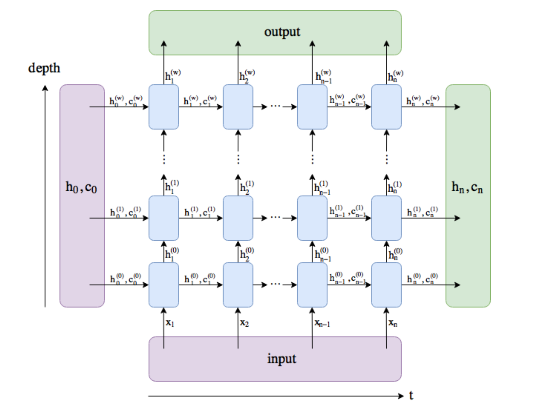
- The horizontal axis or the time axis determines the sequence length or the inputs at various time-steps. The vertical axis determines how many LSTM layers have been stacked together. Beginning from the first layer at the bottom, adding each layer increases the depth of the network. The number of layers are denoted by
win this figure.
- As evident, for each time-step t the LSTM unit takes in $h_{t-1}$, $c_{t-1}$ and $x_{t}$ and gives $h_{t}$ and $c_{t}$. The newly calculated $h_{t}$ and $c_{t}$ are passed to next LSTM unit as hidden and cell state of the sequnce seen so far. Simultaneously $h_{t}$ is also passed as the output for that time-step. This is used as the input for stacked layers above the current layer and finally to calculate predictions. Therefore the
outputof LSTM layer actually contains the hidden states of all time-steps passed through all the layers. Basically, it holds ( $h^{w}_{1}$, $h^{w}_{2}$, ... $h^{w}_{n}$).
- The final hidden and cell states denoted by $h_{n}$ and $c_{n}$ for all the layers are stacked in
(h_n, c_n)output of the LSTM layer. Therefore(h_n, c_n)hold (($h^{1}_{n}$, $c^{1}_{n}$) , ($h^{2}_{n}$, $c^{2}_{n}$) ... ($h^{w}_{n}$, $c^{w}_{n}$)) wherewis number of layers stacked in the LSTM.
INPUT_SIZE = len(review.vocab)
HIDDEN_SIZE = 128
EMBEDDING_DIM = 100
DROPOUT = 0.4
NUM_LAYERS = 1
BIDIRECTIONAL = False
BATCH_SIZE = 64
OUTPUT_DIM = 1
class SentimentLSTM(nn.Module):

    def __init__(self, input_size, hidden_size, embedding_dim, dropout, num_layers, output_dim):

        super().__init__()

        self.embedding = nn.Embedding(num_embeddings=input_size, embedding_dim=embedding_dim)

        self.lstm = nn.LSTM(input_size=embedding_dim, hidden_size=hidden_size, num_layers=num_layers,
                            batch_first=True)

        self.dropout = nn.Dropout(p=dropout)

        self.linear = nn.Linear(in_features=hidden_size, out_features=output_dim)


    def forward(self, x):

        # x = [batch_size, seq_len] = [64, seq_len] as seq_len depends on the batch.

        embed = self.embedding(x)

        # embed = [batch_size, seq_len, embedding_dim] = [64, seq_len, 100]

        # These can be intuitively interpreted as: each example in the batch
        # has a length of seq_len and each word in the sequence is represented
        # by a vector of size 100.

        output, (hidden, cell) = self.lstm(embed)

        # output = [batch_size, seq_len, hidden_size] = [64, seq_len, 128]
        # hidden = [num_layers*num_directions, batch_size, hidden_size] = [1, 64, 128]
        # cell = [num_layers*num_directions, batch_size, hidden_size] = [1, 64, 128]

        # output is the concatenation of the hidden state from every time step,
        # whereas hidden is simply the final hidden state.
        # We verify this using the assert statement.

        output = output.permute(1,0,2)

        # hidden = [1, 64, 128]
        # output = [seq_len, 64, 128]

        assert torch.equal(output[-1,:,:], hidden.squeeze(0))

        preds = self.linear(output[-1,:,:])

        # preds = [64, 1]

        return preds
model = SentimentLSTM(INPUT_SIZE, HIDDEN_SIZE, EMBEDDING_DIM, DROPOUT, NUM_LAYERS, OUTPUT_DIM)
A basic training loop involves the following steps
-
forwardpass, i.e. multiplication of inputs with randomly initialized weights and carrying this on for all the layers. - calculate the
lossof the predictions with the given target/ground truth. - calculate the gradient of the loss function and propagate it
backwardsto calculate gradients of all the layers -
updatingthe weights of all the layers using the gradients so that the objective/loss function converges
def accuracy(preds, y):
    ''' Returns accuracy of the model.'''

    rounded_preds = torch.round(torch.sigmoid(preds))
    correct = (rounded_preds == y).float()
    acc = correct.sum() / len(correct)
    return acc
# define the loss function
criterion = nn.BCEWithLogitsLoss()
# determine the gradient descent algorithm to be used for updating weights
optimizer = optim.SGD(model.parameters(), lr = 1e-3)
# put model and loss on GPU
model = model.to(device)
criterion = criterion.to(device)
The following function performs the training and evaluation simultaneously. Each line has been well documented.
def fit(model, criterion, optimizer, train_iterator, valid_iterator):

    # define number of epochs
    epochs = 3

    # go through each epoch
    for epoch in range(epochs):
        # put the model in training mode
        model.train()
        # initialize losses and accuaracy for every epoch
        train_loss = 0.
        train_acc = 0.
        valid_loss = 0.
        valid_acc = 0.
        print("Epoch: ", epoch)

        # go through each batch from the dataset
        for batch in train_iterator:
            # calculate model predictions. squeeze(1) is done because the output of model is [64,1].
            # criterion expects it to be of dimension [64].
            preds = model(batch.text).squeeze(1)
            # calculate loss for the batch
            loss = criterion(preds, batch.label)
            # add batch loss to total loss for the epoch
            train_loss += loss.item()
            # calculate accuracy for the batch
            train_acc += accuracy(preds, batch.label).item()
            # backward prop for loss function and calc gradients of all the layers in the net
            loss.backward()
            # update the weights
            optimizer.step()
            # make the gradients zero before next step so that they don't accumulate
            optimizer.zero_grad()

        # print recorded results. Divide the total epoch loss/accuracy by the number of examples.
        print('Training loss: ',train_loss / len(train_iterator))
        print('Training accuracy: ', train_acc / len(train_iterator))

        # put the model in evaluation mode
        model.eval()
        # ensures that gradients are not calculated. Takes less time.
        with torch.no_grad():
            # loop through the valid iterator
            for batch in valid_iterator:
                preds = model(batch.text).squeeze(1)
                loss = criterion(preds, batch.label)

                valid_loss += loss.item()
                valid_acc += accuracy(preds, batch.label).item()

        print('Validation loss: ', valid_loss / len(valid_iterator))
        print('Validation accuracy: ', valid_acc / len(valid_iterator))
        print('-------------------------------------------------------------------------------')
fit(model, criterion, optimizer, train_iterator, valid_iterator)