Introduction

Words are an inseparable part of human lives. We communicate verbally, write letters and mail, and even think using words. We can do all of this because we have an understanding of the intrinsic meaning that each word has. Computers on the other hand are not good at understanding words and hence natural language. But they are good at processing large matrices/tensors of floating point values. Hence, humans have always tried to encode the words using numbers in some way that the computers can comprehend and work on challenging tasks. This encoding is usually called a word embedding. Its basically a vector that represents various features or characteristics of the word across its dimensions.
In this post, I intend to explain in detail the working of two techniques that have been used widely to calculate such word embeddings viz. word2vec and GloVe. There are multiple reasons to write this post.

Most of us know how to use these word embeddings in code and build complex architectures using them. However, we often ignore the details of the model and how these vectors were trained in the first place. It is equally important to understand and appreciate them.
For a long time I had the misconception that word2vec and GloVe are somewhat similar with some tweaks here and there. But there are a lot of fundamental differences in their approaches to calculate word-vectors.

In this post I'll briefly explain word2vec and then move on to GloVe dive deep into the model details.

Word2Vec

word2vec uses a pseudo neural network to calculate continuous vector representations for words. Why pseudo? Because we don't actually use the outputs of the trained neural network. The neural network is trained to perform a pseudo or fake task. The task is formulated as done below.

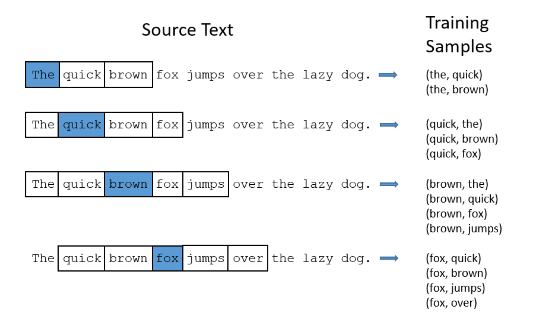
The network is trained using word pairs from large text corpus. For each word in a sentence, we generate word pairs by looking at a fixed number of words before and after the current word (or the input word). This fixed number of words is also known as the window size. This can be 2, 3, 4 or 5. Window size of 3 means that we look at 3 words before and 3 words after the current word $w_{t}$. Which means the context words are ($w_{t-3}$, $w_{t-2}$, $w_{t-1}$, $w_{t+1}$, $w_{t+2}$, $w_{t+3}$). The word-pairs hence generated would be [($w_{t}$,$w_{t-3}$), ($w_{t}$,$w_{t-2}$), ... ($w_{t}$,$w_{t+3}$)]. The word-pairs generated are used to train the network. That is, $w_{t}$ is given as input to the model and the output is one of the words from the context.

Assume that the vocabulary size of the corpus is 10,000. This means that there are 10,000 unique words in the corpus. The input to the network is a one-hot encoded vector representing the input word. The network has one hidden layer with 300 neurons. The output layer has 10,000 neurons, one for each word, with a softmax activation. No activation is used in the hidden layer. The presence of softmax means that the model will actually output probabilities for 10,000 words. This probability is the probability of the word at that index being the nearbuy or a context word for the input/current word. Intuitively, words that occur near the input word multiple times in the corpus will have a larger probability than others.
For example, consider the word "Obama". It is more likely to be surrounded by words like "Barack", "USA", "President" etc. rather than words like "juice", "rabbit" etc. The network hence captures various features of the word statistically by looking at the local context of the word.
Now coming back to the pseudo task. Once this network is trained for all the word pairs in the corpus, we simply remove the output layer. The hidden layer is associated with a matrix of size (10,000 X 300), one 300 dimensional vector for each word in the corpus. After backpropagation, the values of this matrix represent our word vectors. So the proposed task was fake because we never used the output layer. We just wanted to learn representations of the words.

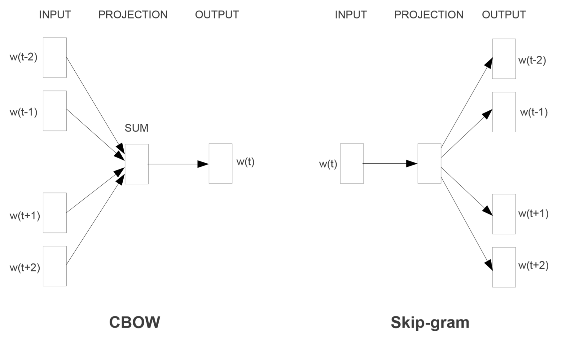
The model discussed above is the skip gram model in which we are predicting the context given the input. The authors also proposed another model in the same paper called continuous bag-of-words (CBOW) model where we predict the input word from the context. A schematic diagram for both these models as given in the paper is shown below

Subsampling

word2vec has been trained on a large corpus extracted from Google News that contains around 100 billion tokens. In such a large corpus, there are bound to exist very high frequency words that contribute very little to the training process. For exxample words like "the", "and", "a" etc. might occur in many context windows and hence be a part of many word-pairs. Thus the authors introduced subsampling that deletes words with high frequency from the corpus. Basically, each word is assigned a probability of whether it will be kept or dropped from the text. For example, if "the" is deleted from a sentence, it will generate fewer word-pairs for training and hence reduce training time.

Negative Sampling

word2vec model has 300 X 10,000 weight values in total. For each training sample, all these weights will get tweaked very slightly. This will happen for all the word-pairs generated in our text. That is, only for one word (ground truth) the output should be 1 and for the rest of the thousand words it should be 0. This would make the training very slow and is not even required since each training sample would not affect the a large fraction of weights significantly. Hence, for each training sample, we choose 5 negative words that we are not present in the input word's context. Weights are tweaked only for the label or the ground truth present in the word pair and these 5 negative words.

Global Vectors (GloVe)

GloVe follows a more principled approach in calculating word-embeddings. The major difference between word2vec and GloVe is that the latter does not use a neural net for the task. The authors develop a strong mathematical model to learn the embeddings. GloVe also overcomes the drawbacks of previous techniques used to calculate word-embeddings. Before word2vec, statistical methods like Latent Semantic Analysis (LSA) were used to approximate embeddings for terms in a document. These methods took into account global count statistics of the dataset. However, the vectors derived from such methods did not capture the meaning of the words like word2vec does and hence performed poorly in tasks like syntactic and semantic similarity and word analogies like "king - queen + woman = man". Meanwhile word2vec took into consideration the local context of words but failed to account for the global count satistics of the dataset. The main aim of GloVe was to combine the two approaches to learn word-vectors. Quoting from the paper,

The statistics of word occurrences in a corpus is the primary source of information available to all unsupervised methods for learning word representations, and although many such methods now exist, the question still remains as to how meaning is generated from these statistics, and how the resulting word vectors might represent that meaning.

Our model efﬁciently leverages statistical information by training only on the non-zero elements in a word-word co-occurrence matrix, rather than on the entire sparse matrix or on individual context windows in a large corpus.

As highlighted above, GloVe derives its training data by calculating a word-word co-occurence matrix. We'll show how this is calculated below with a toy example. But its important to understand the difference between this method and that used by word2vec. Word2vec generated training samples by forming word-pairs for all the words in a local context window completely ignoring the global statistics of the words that occur in the context window.

Co-occurence matrix

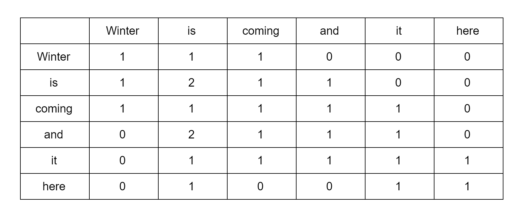
Consider the sentence - "Winter is coming and it is here.". We construct a co-occurence matrix for this sentence with a context window size of 2. For "winter", the context words are "is" and "coming". Hence, we put 1 in the respective box. We also assume that the word itself is part of its context and hence increment the count in the diagonal of the matrix.

Derivation

We'll now get into the derivation of the GloVe model. The following section contains equations taken from the paper directly. Although I'll try my best to explain the significance and meaning of each equation, the derivation can get a bit daunting. Let's start by defining some notations.

Let the word-word co-occurrence table be denoted by $X$. Each entry in the table $X_{ij}$ denotes the number of times word $j$ occurs in the context of word $i$.
Let $X_{i}$ be the number of times any word appears in the context of word $i$. That is the total number of distinct words throughout the corpus that appear in word $i$'s context. Therefore, $X_{i}$ = $\sum_{k}$$X_{ik}$ where $k$ are the different words that appear in $i$'s context throughout the dataset.
Let $P_{ij}$ = $P (j | i)$ = $X_{ij}$ / $X_{i}$. This defines the probability that word $j$ appears in the context of word $i$. $P_{ij}$ is also called as the co-occurrence probability.

By calculating this probability, we are actually incorporating the global statistics of the dataset. Word2vec ignores the denominator of $P_{ij}$ calculated above.

Consider the following calculations for a particular dataset. The following example will help us understand how can we derive meaning of words by the ratio of probabilities calculated above.

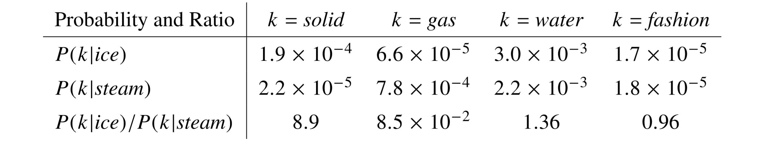
The above matrix shows raw probabilities and ratios for two words viz. ice and steam. These words are topically concerned with the thermodynamic phases of water. The first 2 rows show calculations of the the probability $P_{ik}$ where $k$ are some words from the dataset called probe words. The last row shows the ratio of probabilities calculated in the first two rows. The hypothesis is as follows:

The relationship of these words can be examined by studying the ratio of their co-occurrence probabilities with various probe words, $k$.

Among the probe words, "solid" is closely related to the word "ice" (word $i$) and "gas" is closely related to "steam" (word $j$). As can be seen in the table above, the ratio $P_{ik}$/$P_{jk}$ is much greater than 1 (8.9) for words that are similar to "ice" ($i$) and much smaller than 1 (0.085) for words that are related to "steam" ($j$). Moreover, for words that are equally related to both "ice" and "steam" like "water" and words that not related to any off the two words (like "fashion") have the ratio around 1.
Therefore, the hypothesis stated above is true in the sense that ratios of co-occurrence probabilities gives a better sense about the meaning of a word than raw probabilities.

Therefore, this seems to be a good starting point for learning word vectors. We need to learn a function $F$, parameterized by 3 word vectors $w_{i}$, $w_{j}$ and $\tilde w_{k}$ such that,

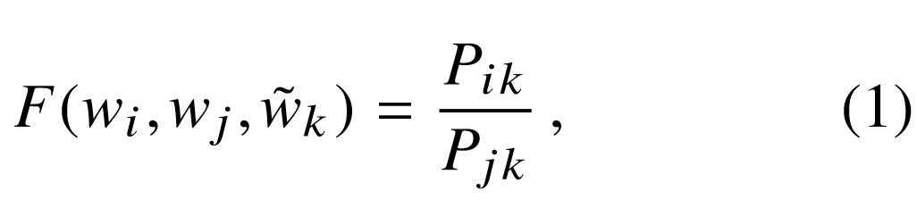
$w_{i}$, $w_{j}$ and $\tilde w_{k}$ belong to $R^{ d}$. $\tilde w_{k}$ represent separate context words or the probe words as discussed above.

There are a large number of possibilities for the function $F$. So lets impose some constraints on the model. The purpose of this model is to learn embeddings or feature vectors for words. Once learned, these vectors can be projected into a vector space just like we project 2 and 3 dimensional vectors in a cartesian plane. These vector spaces are inherently linear in nature because a vector is ultimately just a line.
The above discussion leads us to our first constraint. The most common way to compare two linear structures is to calculate their difference. Thus we can restrict our function as,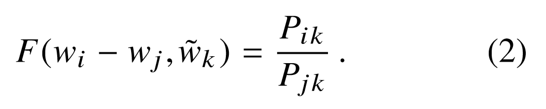

In the above equation, the right hand side is a ratio which is scalar and the arguments are vectors. While, learning a complex function $F$ that does the above mapping is possible but that would introduce non-linearities in our model because that's what neural nets do. We don't wish to obscure the linear structure that our model captures. Therefore, we take a dot product of the arguments on the left hand side to make it a scalar.

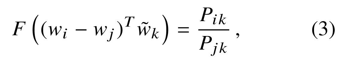
The next constraint is that of symmetry. The distinction between a word and the context words is arbitary and hence they can be exchanged with each other. This is easy to understand. If "water" and "gas" can be used as context words for "steam", then "steam" can also be used as a context word for "water" and "gas". This symmetry is also evident in our co-occurrence matrix $X$ which is symmetric about the diagonal. Symmetry implies that $w$ $<->$ $\tilde w$. To restore this symmetry, we require that the function $F$ is a homomorphism between groups $(R, +)$ and $(R_{>0}, *)$.

Let's define a group and homomorphism.
A group $(G, *)$ is set of elements, that is closed under a particular operation $*$. That is if $x$ and $y$ belong to $G$ then, $z$ = $x$ $y$ also belongs to $G$. Each group has an inverse such that for all $x$, $x^{-1}x$ = $e$. Also, for all elements in a group, there exists an identity such that $xe = ex$ = $x$. Function $F$ is a homomorphism between 2 groups $(G, )$ and $(H, @)$ such that $F:G ->H$ if $F(xy) = F(x) @ F(y)$.

Coming back to the equation of the model, homomorphism for $F$ can be explained as

\begin{equation} F((w^{T}_{i} - w^{T}_{j})\tilde w_{k}) = F(w^{T}_{i}\tilde w_{k} + (-w^{T}_{j}\tilde w_{k})) \end{equation}\begin{equation} F(w^{T}_{i}\tilde w_{k} + (-w^{T}_{j}\tilde w_{k})) = F(w_{i}^{T} \tilde w_{k}) * F(-w_{j}^{T} \tilde w_{k}) \end{equation}\begin{equation} F(w_{i}^{T} \tilde w_{k}) * F(-w_{j}^{T} \tilde w_{k}) = F(w_{i}^{T} \tilde w_{k}) * F(w_{j}^{T} \tilde w_{k})^{-1} \end{equation}

The above equation gives the following result,

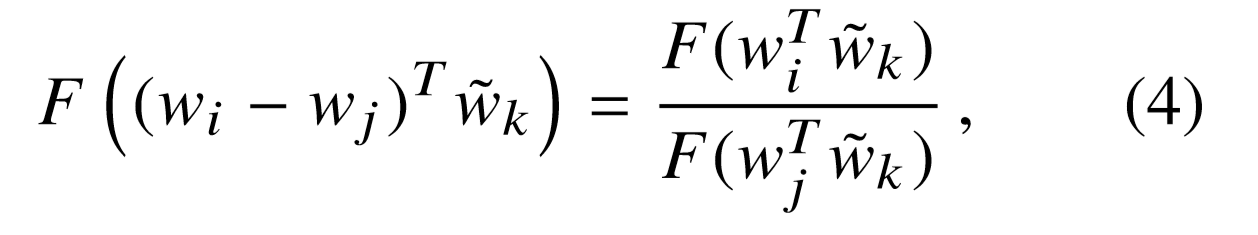
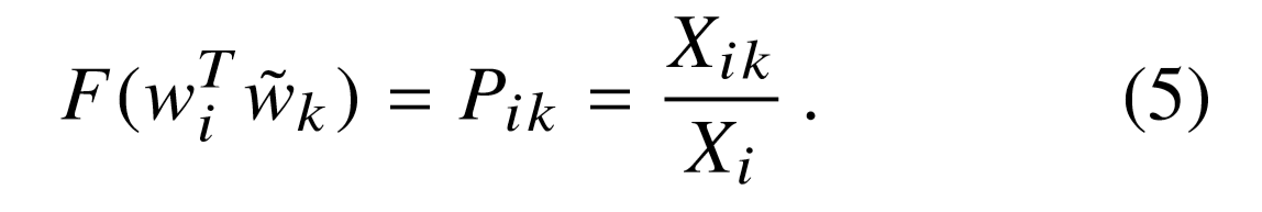
The above equation is solved by equation $(3)$,

And the exponential function is the solution for equation $(4)$, therefore we have the following,

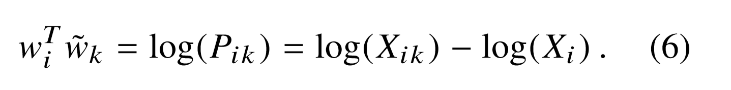
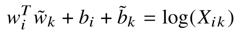
he symmetry is still not restored because of the $log(X_{i})$ term on the right hand side. Since, this term is independent of $k$, we can absorb it into bias $b_{i}$. Also introducing a bias $\tilde b_{k}$ for $\tilde w_{k}$, we finally have the following equation,

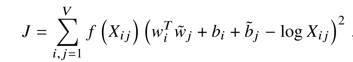
The above equation gives us a cost function for a new weighted least squares regression model. The weighting function $f(X_{ij})$ takes into consideration the co-occurrences of words.

References and Acknowledgements

This post is heavily derived from the respective research papers of the techniques. Figures and equations are taken from the papers and blogs referenced below. Chris McCormick's posts on word2vec are still the best explanations for the topic and I strongly recommend the reader to read those.